Create View Graph Using Bag of Features
This example shows how to build a view graph from a collection of images using an feature-based (bag-of-features) similarity search. A view graph is a graph where each node represents an image and each edge indicates that two images are likely to see overlapping scene content. View graphs are often used as a starting point for Structure from Motion (SfM) [1] and visual SLAM pipelines. They help identify candidate image pairs for initialization before applying further steps like geometric verification and camera pose estimation.
Download Images
This example uses a subset of the TUM RGB-D Benchmark [2] containing 104 images of a indoor office scene. You can download the data to a temporary directory using a web browser or by running the following code:
% Location of the compressed data set
url = " https://ssd.mathworks.com/supportfiles/3DReconstruction/tum_rgbd_data.zip";

% Store the data set in a temporary folder
downloadFolder = tempdir;
filename = fullfile(downloadFolder, "tum_rgbd_data.zip");

% Uncompressed data set
imageFolder = fullfile(downloadFolder, "sfmTrainingDataTUMRGBD", "images");

if ~exist(imageFolder, "dir") % download only once
disp('Downloading TUM RGB-D Dataset (119 MB)...');
    websave(filename, url);
    unzip(filename, downloadFolder);
end
Create an imageDatastore to manage the images. The images are ordered in time, but the SfM pipeline demonstrated in the example also supports non-sequential images.
imds = imageDatastore(imageFolder);
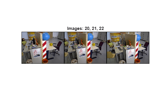
Inspect a few sample images to understand the scene's content and viewpoint variation.
imageIdx =22; im1 = readimage(imds,imageIdx-2); im2 = readimage(imds,imageIdx-1); im3 = readimage(imds,imageIdx); figure montage({im1,im2,im3}, Size=[1 3], BorderSize=4) title("Images: " + num2str(imageIdx-2) + ", " + (imageIdx-1) + ", " + imageIdx)
Find Similar Image Pairs
Appearance-based search proposes candidate image pairs for downstream geometric verification. Each image is represented by Local Feature Detection and Extraction and their descriptors, which are a compact vector representations of a local neighborhood. A recognition database is used to retrieve the most similar images for each query image [3]. These similar image pairs are added as edges in the view graph, connecting images that are likely to observe overlapping parts of the scene.
This example uses ORB features because the dbowLoopDetector object provides a built-in ORB-based vocabulary. This avoids the need to train a custom vocabulary, which can be time-consuming and computationally expensive.
This example uses the imageviewset function to create a view graph.
% Create an image view set to store views and later connections
viewGraph = imageviewset();

% Get the number of images in the data set
numImages = numel(imds.Files);

% Pre-allocate cells to store features and keypoints features
featuresORB    = cell(1,numImages);
validPointsORB = cell(1,numImages);
for viewId = 1:numImages
    % Read image
    colorI = readimage(imds,viewId);

    % Convert image to grayscale
    I = im2gray(colorI);

    % Detect ORB keypoints
    points = detectORBFeatures(I);

    % Extract ORB descriptors at detected keypoints
    [featuresORB{viewId},validPointsORB{viewId}] = extractFeatures(I, points);

    % Add the view to the view graph
    viewGraph = addView(viewGraph, viewId);
end
Initialize the loop detector and build the recognition database. Add the ORB features from each image to the database using the image’s view identifier.
% Create a recognition database with a default ORB vocabulary
loopDetector = dbowLoopDetector();

% Add features for each view to the recognition database
for viewId = 1:numImages
    addVisualFeatures(loopDetector, viewId, featuresORB{viewId});
end
For each query image, retrieve its visually most similar images by features and add connections to the view graph. A typical number for similar images is from 10 to 30. For this small dataset, the value is set to 10. To reduce downstream computation in SfM, add uni-directional connections from each query image to its nearest neighbors rather than forming all bi-directional pairs.
% Number of most similar images per query image
numSimilarImages = 10;

% For each query image, retrieve the top-k most similar images
% and add appearance-based connections to the view graph
for queryId = 1:numImages

    % Use the loopDetector to retrieve the IDs of the nearest matches to
    % the query image in the dataset
    loopViewIds = detectLoop(loopDetector, featuresORB{queryId}, NumResults=numSimilarImages+1);

    % Remove the query image from the candidate list if present
    neighborIds = setdiff(loopViewIds, queryId);

    % Add connections from the query image to its similar images
    % Use uni-directional connections to reduce downstream computation
    for i = 1:numel(neighborIds)
        connectioNotExists = ~hasConnection(viewGraph, queryId, neighborIds(i)) && ...
            ~hasConnection(viewGraph, neighborIds(i), queryId);
        if connectioNotExists
            viewGraph = addConnection(viewGraph, queryId, neighborIds(i));
        end
    end
end
Visualize View Graph
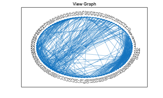
To assess overall connectivity, plot the nodes and edges in the view graph and visualize the adjacency matrix. The view graph indicates that each image is connected to its nearby images, as expected for a sequential dataset. A few long-range connections appear; these are likely outliers and will be pruned during geometric verification.
G = createPoseGraph(viewGraph);
figure
plot(G, NodeLabel=1:numImages, Layout="circle");
title("View Graph");
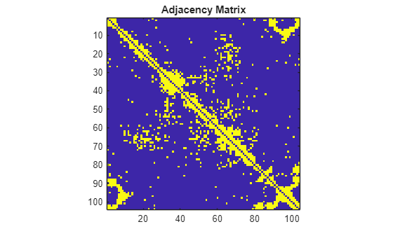
The adjacency matrix provides a per-image view of similarity. The dense blocks correspond to the images with small camera motion and high scene overlap. The early images connect to the later ones, indicating the camera eventually returns to its starting area.
% Get adjacency matrix from the view graph
A = adjacency(G);

% Convert the adjacency matrix to a symmetric matrix for clearer
% visualization of mutual connectivity
A = A+A';
figure
imagesc(A)
axis image
title("Adjacency Matrix");
Visualize Similar Images
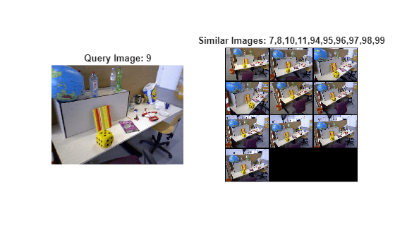
The following visualization shows the nearest images for a selected query in the view graph. In addition to true similar images that share overlapping content, spurious matches may be present because no geometric verification is performed at this stage and we rely solely on visual appearance based on local feature similarity.
% Select a query image and inspect its connected images queryIdx =9; viewTable = connectedViews(viewGraph, queryIdx); similarIdx = viewTable.ViewId; queryImg = readimage(imds, queryIdx); retrievedImages = cell(numel(similarIdx),1); for i = 1:numel(similarIdx) retrievedImages{i} = readimage(imds, double(similarIdx(i))); end figure subplot(1,2,1) imshow(queryImg) title("Query Image: " + queryIdx) subplot(1,2,2) montage(retrievedImages, BorderSize=5) title("Similar Images: " + strjoin(string(similarIdx), ","))
Match Features Between Similar Images
After the view graph is created, the next step is to perform feature matching between each connected image pair in the view graph. You can use ORB descriptors extracted earlier but SIFT descriptors provide more reliable matching quality and downstream accuracy along the SfM pipeline. To use SIFT descriptors, update each view in the view graph with SIFT features.
for viewId = 1:numImages
    % Read and convert image to grayscale
    I = im2gray(readimage(imds, viewId));

    % Detect SIFT keypoints. Use a smaller ContrastThreshold value
    % to detect more points.
    points = detectSIFTFeatures(I, ContrastThreshold=0.0067);

    % Extract SIFT descriptors at detected keypoints
    [featuresSIFT, validPointsSIFT] = extractFeatures(I, points);

    % Update the views in the view graph with feature points and
    % feature descriptors
    viewGraph = updateView(viewGraph, viewId, rigidtform3d, ...
        Points=validPointsSIFT, Features=featuresSIFT);
end
For each pair of similar images, use descriptor matching to identify feature correspondences. The following loop performs SIFT matching with a ratio test and stores the results in the graph. Increasing maxRatio and matchThreshold will yield more matched pairs, but also more outliers. Note that this step performs feature descriptor matching only and does not include geometric verification.
% Get the view IDs for all the connections
viewIds1 = viewGraph.Connections.ViewId1;
viewIds2 = viewGraph.Connections.ViewId2;
numConnections = viewGraph.NumConnections;

% Set parameters for feature matching
maxRatio      = 0.8;
matchTheshold = 40;

for connId = 1:numConnections
    % Get view IDs of the two images
    viewId1   = viewIds1(connId);
    viewId2   = viewIds2(connId);

    % Get the features from the two images
    view1     = findView(viewGraph, viewId1);
    view2     = findView(viewGraph, viewId2);
    features1 = view1.Features{:};
    features2 = view2.Features{:};

    % Match SIFT features between the two images and apply ratio check
    indexPairs = matchFeatures(features1, features2, ...
        MaxRatio=maxRatio, MatchThreshold=matchTheshold, Unique=true);

    % Update the connection with matched pairs of features
    viewGraph = updateConnection(viewGraph, viewIds1(connId), viewIds2(connId), ...
        rigidtform3d, Matches=indexPairs);
end
Visualize Matched Features
Because the matching is based solely on feature descriptors, the matched points are not guaranteed to correspond to the same 3-D scene points. The visualization below examines matches for a selected image pair: a feature in one image may be paired with a feature in the other image that does not belong to the same physical part of the scene.
% Pick one of the image pairs and visualize the matched features connId =143; matchedPairs = viewGraph.Connections.Matches{connId}; viewId1 = viewIds1(connId); viewId2 = viewIds2(connId); view1 = findView(viewGraph, viewId1); view2 = findView(viewGraph, viewId2); points1 = view1.Points{:}; points2 = view2.Points{:}; % Get the matched SIFT points matchedPoints1 = points1(matchedPairs(:,1)); matchedPoints2 = points2(matchedPairs(:,2)); % Read image pair I1 = readimage(imds, viewId1); I2 = readimage(imds, viewId2); figure showMatchedFeatures(I1, I2, matchedPoints1, matchedPoints2, "montage", PlotOptions={"ro","g+","y--"}); truesize
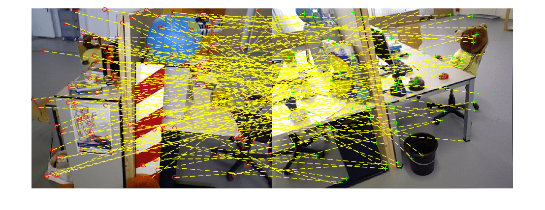
These matches should be verified by estimating a 2-D transform that maps features points between images. This is done by using epipolar geometry (e.g., fundamental matrix) or projective geometry (e.g., homography), combined with robust estimation techniques like RANSAC to filter out outliers. For a complete example showing geometric verification of matched features in the view graph, see Refine View Graph Using Geometric Verification.
References
[1] Schonberger, Johannes L., and Jan-Michael Frahm. "Structure-from-motion revisited." In Proceedings of the IEEE conference on computer vision and pattern recognition, pp. 4104-4113. 2016.
[2] Sturm, Jürgen, Nikolas Engelhard, Felix Endres, Wolfram Burgard, and Daniel Cremers. "A benchmark for the evaluation of RGB-D SLAM systems". In Proceedings of IEEE/RSJ International Conference on Intelligent Robots and Systems, pp. 573-580, 2012.
[3] Gálvez-López, Dorian, and Juan D. Tardos. "Bags of binary words for fast place recognition in image sequences." IEEE Transactions on robotics 28, no. 5 (2012): 1188-1197.
See Also
imageviewset | detectORBFeatures | detectSIFTFeatures | dbowLoopDetector | createPoseGraph