Run ArduPilot Software-in-the-Loop Simulation with Fixed-Wing Plant in Simulink

R2026b

Since R2026b

This example shows you how to verify a fixed-wing controller design, by using software-in-the-loop (SITL) simulation, and to simulate the fixed-wing plant model in Simulink using the UAV Toolbox Support Package for ArduPilot® Autopilots.

Prerequisites

• Simulink — If you are new to Simulink, watch the Simulink Quick Start video.

• UAV Toolbox Support Package for ArduPilot Autopilots in Windows® — If the support package is not already installed, follow the steps in Install UAV Toolbox Support Package for ArduPilot Autopilots in Windows. At the Select an ArduPilot Board step of installation, specify these options:

Autopilot name — ArduPilot Host Target

Board — sitl

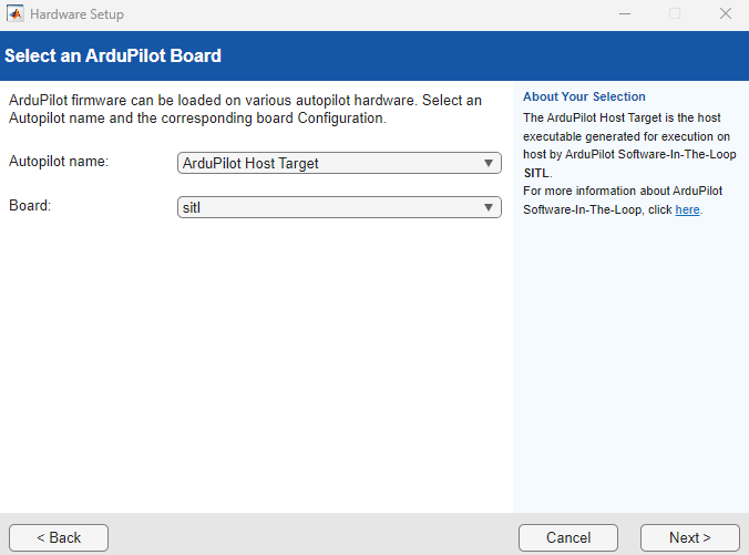
If you have already installed the support package, open the hardware setup screen and verify that Autopilot name is set to ArduPilot Host Target and Board is set to sitl.

Launch First MATLAB Instance

Launch the first instance of MATLAB. To access the Simulink model, supporting files, and project shortcuts that this example uses, open the ArduPlaneSITLSimulinkPlant.prj project file.

prj = openProject("ArduPlaneSITLSimulinkPlant");

Copy the current folder path of the first MATLAB instance to the clipboard.

clipboard("copy", pwd)

Fixed-Wing Dynamics Model Overview

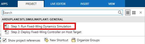
To open the fixed-wing Plane_UAV_Dynamics.slx Simulink model, on the Project tab of the MATLAB Toolstrip, in the Shortcuts section, click the Step 1: Run Fixed-Wing Dynamics Simulation shortcut.

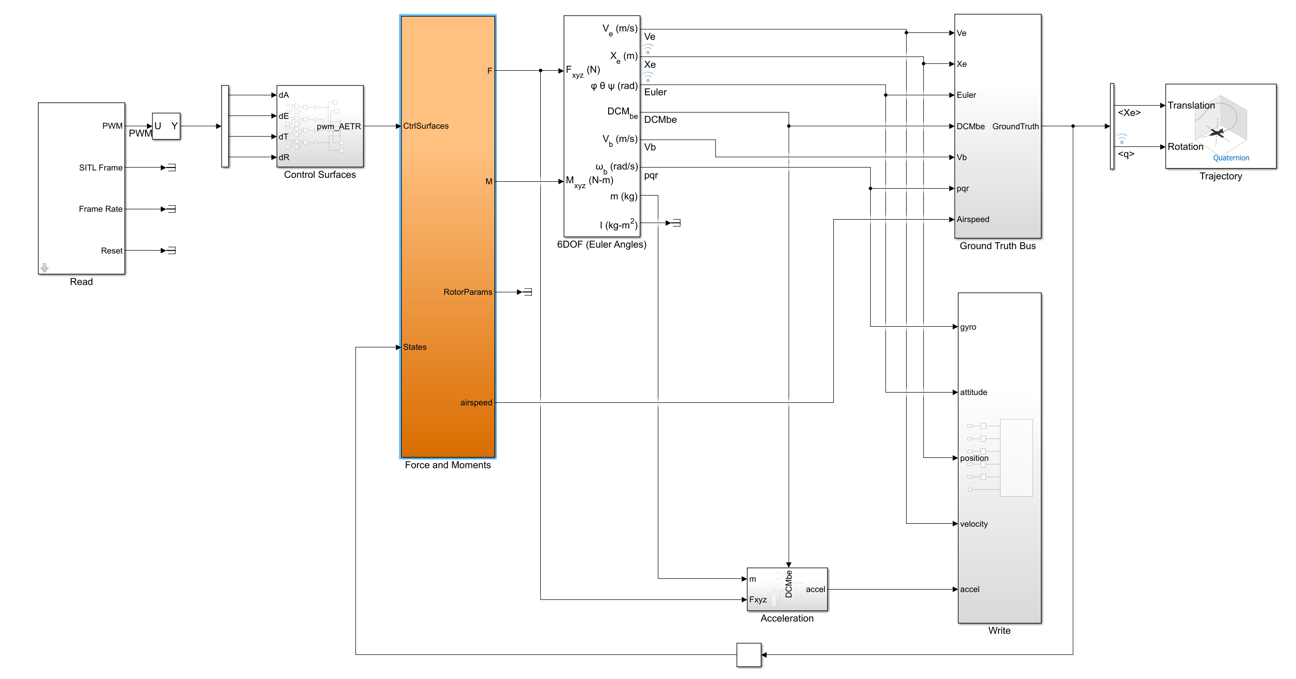
The Plane_UAV_Dynamics.slx Simulink model contains these main blocks and subsystems:

• Read subsystem — Reads the PWM signals sent by the ArduPilot host target through a UDP connection.

• Control Surfaces subsystem — Converts the PWM signals to control surface deflections.

• Force and Moments subsystem — Calculates the forces and moments generated by the aerodynamics, propulsion system, gravity, and ground contact models based on the motor angular velocity and fixed-wing states. The subsystem passes the calculated forces and moments to the 6DOF (Euler Angles) block as inputs.

• 6DOF (Euler Angles) (Aerospace Blockset) block — Calculates the fixed-wing states of the UAV by using six-degrees-of-freedom equations of motion.

• Write subsystem — Sends the fixed-wing states to the ArduPilot host target through a UDP connection.

Run Fixed-Wing Plant Model in First MATLAB Instance

Get the IP address Windows uses to connect to the virtual network of the Windows Subsystem for Linux (WSL) instance running the ArduPilot flight stack. First, open the Windows Command Prompt. Then, at the command line, enter ipconfig and locate the entry for Ethernet adapter vEthernet (WSL (Hyper-V firewall)). The IP address of Windows on the virtual network is the IPv4 Address, which in this example is 172.21.176.1.

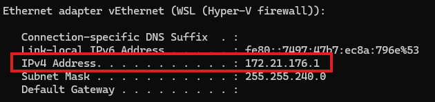
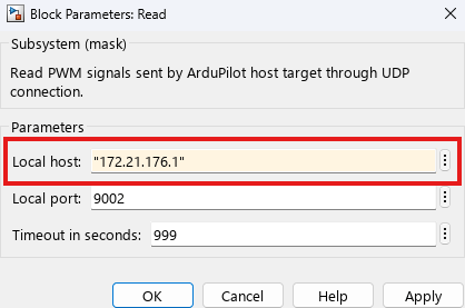
In the Plane_UAV_Dynamics.slx model, open the block mask of the Read subsystem. Specify the Local host parameter as the IP address of Windows on the WSL virtual network, and specify the Local port parameter as 9002. Click OK to save the changes.

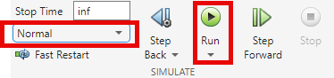
On the Simulation tab of the Simulink Toolstrip, in the Simulate section, select the Normal simulation mode. Then, to start the Plane_UAV_Dynamics.slx model, click Run .

For more information on connecting MATLAB to ArduPilot SITL, see the MATLAB Simulation section of the ArduPilot documentation.

Launch Second MATLAB Instance

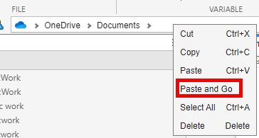
Launch a second instance of MATLAB. Then, right-click the current working directory in the address bar context menu and paste the folder path of the first instance of MATLAB by selecting Paste and Go.

To access the Simulink model, supporting files, and project shortcuts that this example uses, open the ArduPlaneSITLSimulinkPlant.prj project file.

prj = openProject("ArduPlaneSITLSimulinkPlant");

Fixed-Wing Controller Model Overview

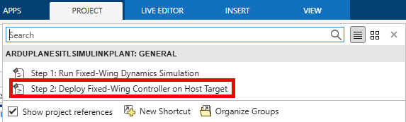
To open the Plane_Controller.slx Simulink model, on the Project tab of the MATLAB Toolstrip, in the Shortcuts section, click the Step 2: Deploy Fixed-Wing Controller on Host Target shortcut.

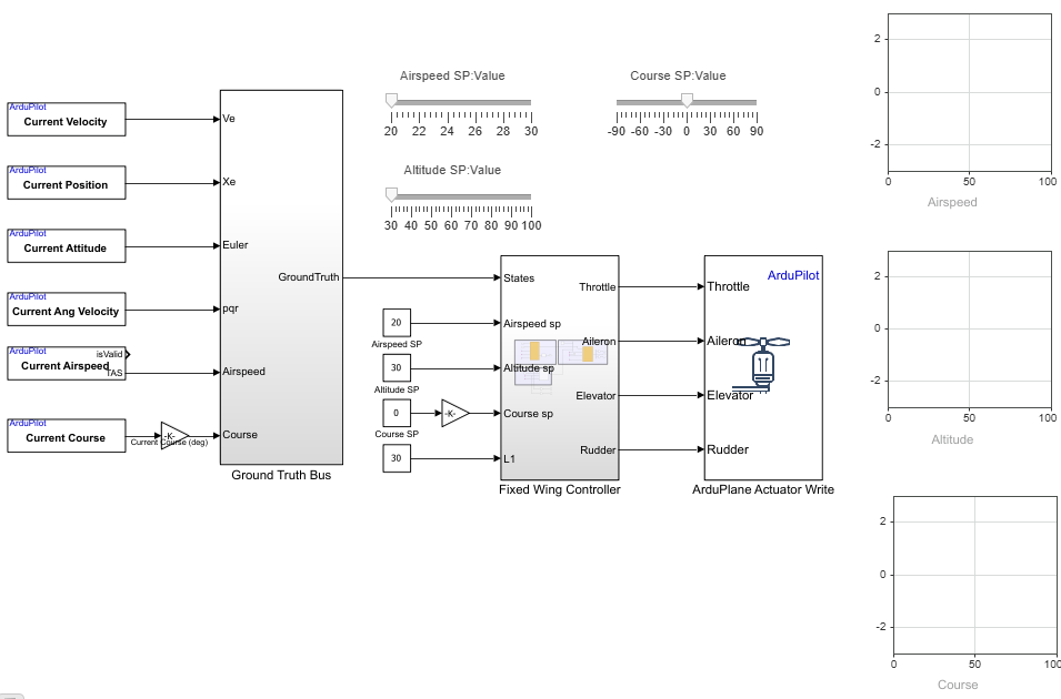
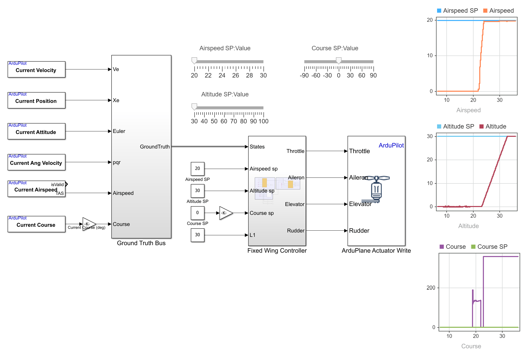
The Fixed Wing Controller subsystem calculates the normalized throttle and servo actuator setpoints, which it passes to the ArduPlane Actuator Write block as inputs. The ArduPlane Actuator Write block writes normalized throttle and servo commands to the throttle, aileron, elevator, and rudder of the UAV.

The Fixed Wing Controller subsystem obtains the airspeed, altitude, and course setpoints from Constant blocks, which you can adjust using the Airspeed SP:Value, Altitude SP:Value, and Course SP:Value sliders, respectively, during simulation. The subsystem also accepts the L1 distance, which specifies the distance of the lookahead point used by the lateral controller.

The Fixed Wing Controller subsystem obtains state feedback from the Ground Truth Bus subsystem, which aggregates feedback from these blocks:

• Current Position — Outputs the current UAV position.

• Current Velocity — Outputs the current UAV velocity.

• Current Attitude — Outputs the current attitude of the UAV.

• Current Ang Velocity — Outputs the current angular velocity of the UAV.

• Current Airspeed — Outputs the current airspeed of the UAV.

• Current Course — Outputs the current course of the UAV.

To visualize the simulation result, the Plane_Controller Simulink model uses Dashboard Scope (Simulink) blocks that visualize the setpoint and feedback signals for airspeed, altitude, and course.

Fixed Wing Controller Subsystem

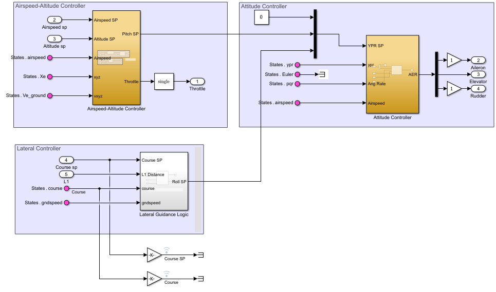
The Fixed Wing Controller subsystem contains the Airspeed-Altitude Controller, Lateral Guidance Logic, and Attitude Controller subsystems.

Airspeed-Altitude Controller Subsystem

The Airspeed–Altitude Controller subsystem calculates the throttle and pitch setpoints based on airspeed and altitude tracking errors. It uses PID Controller (Simulink) blocks to generate throttle and pitch commands that enable the UAV to maintain the specified airspeed and altitude.

Lateral Guidance Logic Subsystem

The Lateral Guidance Logic subsystem calculates the roll setpoint, which it passes to the Attitude Controller subsystem as input. The Lateral Guidance Logic subsystem uses the L1 guidance law to determine the required lateral acceleration based on the current course, course setpoint, ground speed, and distance to the lookahead point [1].

Attitude Controller Subsystem

The Attitude Controller subsystem computes normalized aileron, elevator, and rudder commands to track the commanded roll, pitch, and yaw. It uses PID controllers to regulate attitude and angular rates, and includes a turn‑coordination algorithm implemented in a MATLAB Function block to compute the rudder command required for coordinated, no‑slip flight.

Verify Hardware Settings

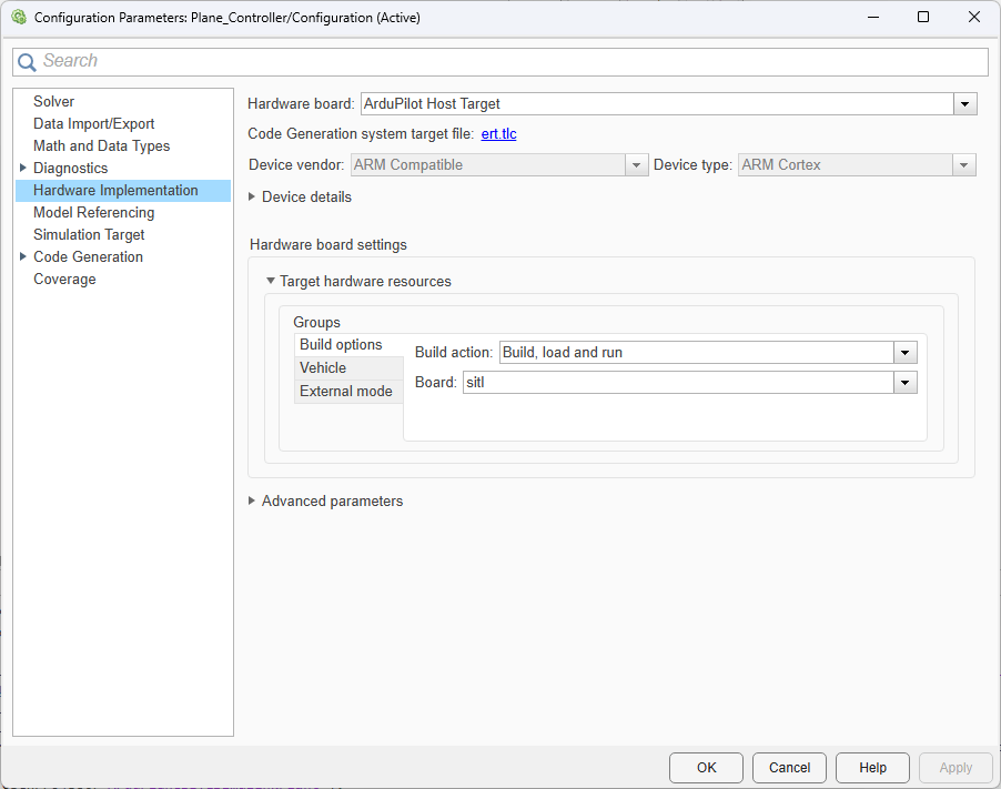
On the Simulink Toolstrip of the Plane_Controller.slx model, on the Hardware tab, click Hardware Settings . In the left pane, select Hardware Implementations, and verify these options:

• Hardware board is set to ArduPilot Host Target.

• In the Hardware board settings section, under Target hardware resources, select the Build options tab of the Groups pane. Verify that Build action is set to Build, load and run, and Board is set to sitl.

• Select the Vehicle tab of the Groups pane. Verify that Simulator is set to Simulink.

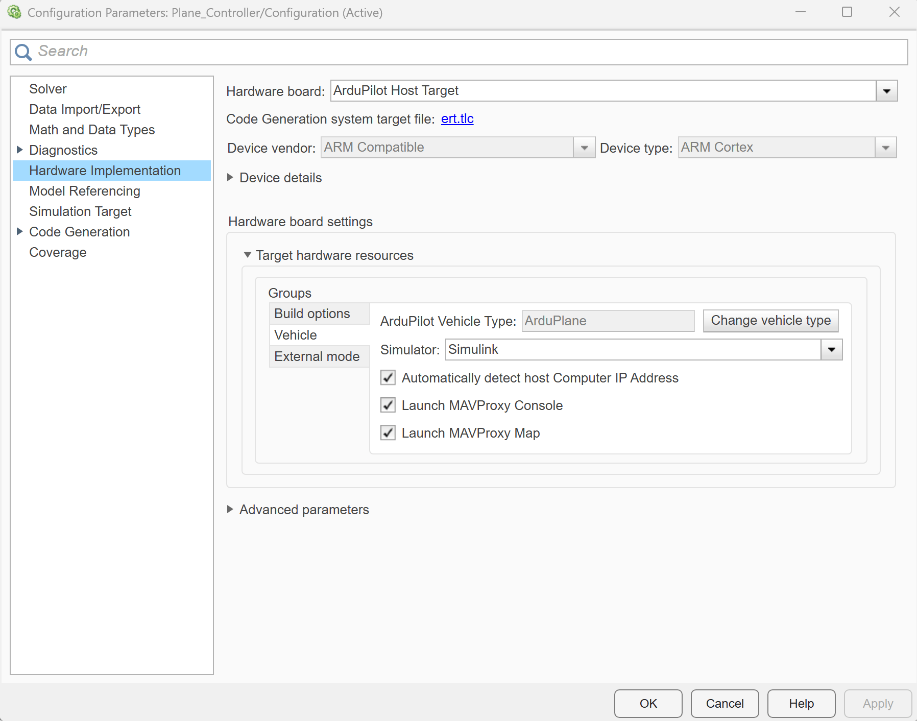
Click OK to save any changes and close the Configuration Parameters dialog box.

Run Fixed-Wing Controller Model in Second MATLAB Instance

To run the Plane_Controller.slx model in Monitor & Tune mode:

1. From the Simulink Toolstrip, select the Hardware tab.

2. Verify that the Mode section contains a Run on board button. If it instead contains a Connected IO button, click Connected IO, then Run on board (External mode).

3. In the Run on Hardware section, click Monitor & Tune .

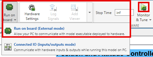
Start Simulation

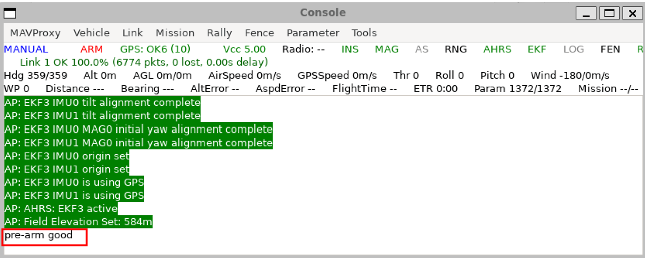
The MAVProxy console and Windows terminal launch after you run both Simulink models. Wait until the MAVProxy console shows the message pre-arm good before proceeding to the next step.

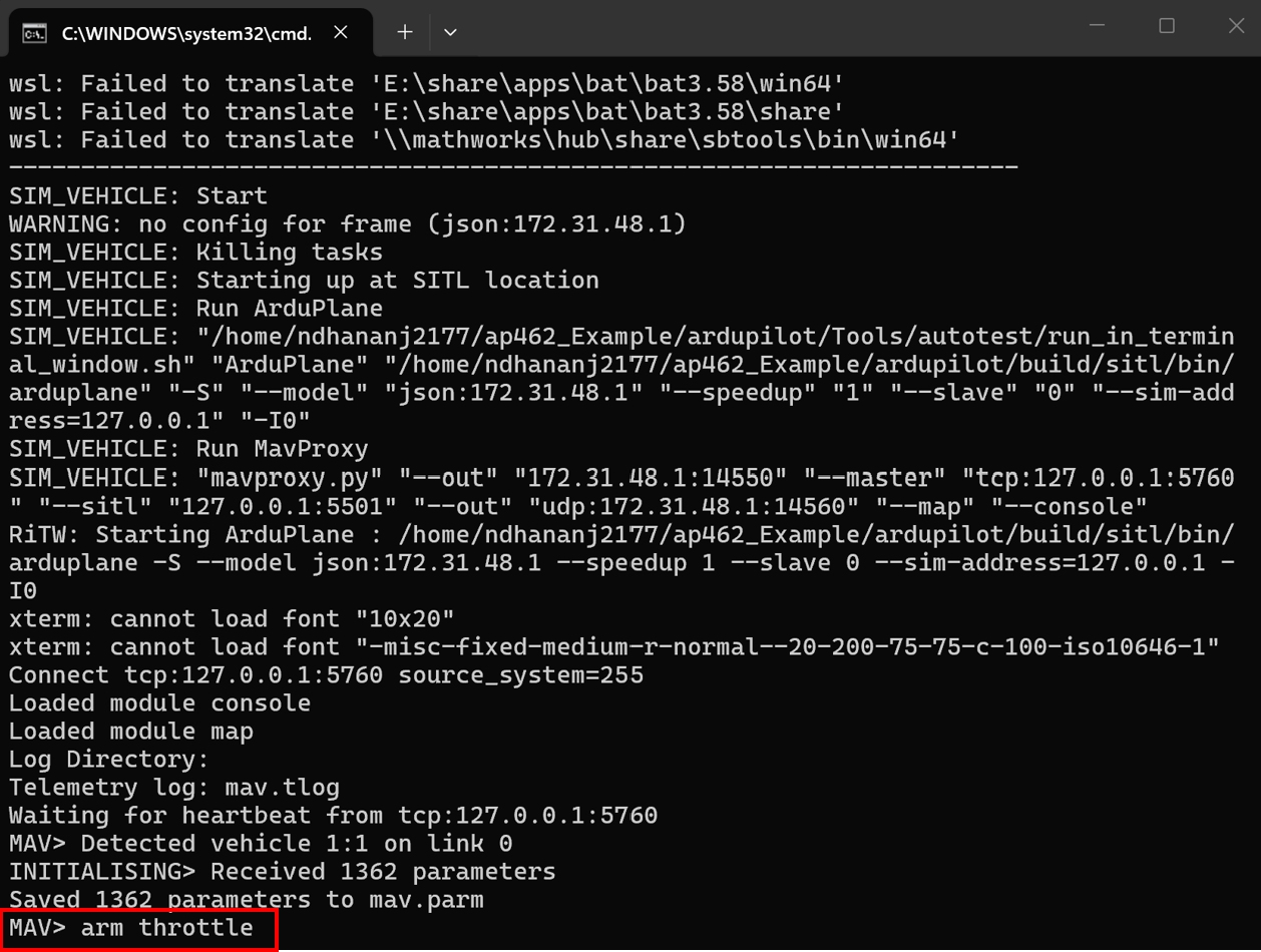
Arm the UAV by entering the command arm throttle in the Windows terminal.

After arming is complete, the UAV takes off and reaches the specified altitude and airspeed. You can then change the setpoints using the sliders. Use the sliders to adjust the airspeed, altitude, and course. The dashboard scope displays both the setpoints and the actual signal values.

To end the simulation after the mission has finished, first stop the Plane_UAV_Dynamics.slx Simulink model, then stop the Plane_Controller.slx Simulink model. If you instead stop the Plane_Controller.slx Simulink model first, then you must press Ctrl+C to stop the Plane_UAV_Dynamics.slx Simulink model.

References

[1] Park, Sanghyuk, John Deyst, and Jonathan How. “A New Nonlinear Guidance Logic for Trajectory Tracking.” Paper presented at AIAA Guidance, Navigation, and Control Conference and Exhibit, Providence, Rhode Island. AIAA Guidance, Navigation, and Control Conference and Exhibit, American Institute of Aeronautics and Astronautics, August 16, 2004. https://doi.org/10.2514/6.2004-4900.