Empirical Distribution

The empirical distribution is a nonparametric estimate of the cumulative distribution function (cdf) for a sample. As the sample size increases, the empirical distribution cdf converges to the cdf of the distribution from which the sample was taken. The empirical distribution is useful for analyzing samples when the underlying probability distribution is unknown, and is often used for bootstrap resampling.

Statistics and Machine Learning Toolbox™ offers multiple ways to work with the empirical distribution:

• Create a probability distribution object EmpiricalDistribution by specifying parameter values using fitdist. Then, use object functions to evaluate the distribution, generate random numbers, and so on.

• Use the distribution-specific function ecdf with a data sample to evaluate its empirical cdf at a vector of points or a matrix of intervals. Use the ecdfhist function to calculate heights and bin centers for an empirical cdf.

Cumulative Distribution Function

For a sample with n observations, the cumulative distribution function (cdf) is a step function that increases by 1/n at each observation with a unique value. If k observations have the same value, the cdf increases by k/n at that value. The cdf is given by the equation

$$p(x_i)=\frac{i}{n}$$

where i is the number of observations with values less than or equal to x_i.

Examples

Fit Empirical Distribution to Data

Generate random data from a standard normal distribution. Visualize the data x using a histogram.

rng("twister") % For reproducibility
mu = 0;
sigma = 1;
normalpd = makedist("Normal");
x = random(normalpd, [100 1]);
histogram(x)

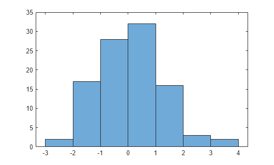
The histogram has a typical bell shape with a single mode.

Create an empirical probability distribution object by using fitdist to fit an empirical distribution to the same data x. The object contains various distribution properties, such as the evaluation points (X), cdf values (FX), and InputData.

empiricalpd =  fitdist(x,"Empirical");
properties(empiricalpd)

Properties for class prob.EmpiricalDistribution:

    DistributionName
    X
    FX
    Truncation
    IsTruncated
    InputData

Plot the evaluation points X and the cdf values FX.

figure
plot(empiricalpd.X,empiricalpd.FX)
hold on

Superimpose the empirical cdf returned by the ecdf function.

empiricalCdf = ecdf(empiricalpd.X);
plot(empiricalpd.X,empiricalCdf)
hold on

Superimpose the normal cdf.

normalCdf = cdf(normalpd,empiricalpd.X);
plot(empiricalpd.X,normalCdf)
legend("FX from empirical distribution object","Empirical cdf from ecdf","Known population (normal) cdf", ...
    "Location","southeast")
hold off

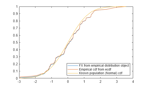
The plot shows that ecdf and FX follow each other closely. The empirical cdf also closely follows the normal distribution cdf.

Compute Empirical cdf

Compute the Kaplan-Meier estimate of the empirical cumulative distribution function (cdf) for simulated survival data.

Generate survival data from a Weibull distribution with parameters 3 and 1.

rng("default")  % For reproducibility
failuretime = random("wbl",3,1,15,1);

Compute the Kaplan-Meier estimate of the empirical cdf for the survival data.

[f,x] = ecdf(failuretime);
[f,x]

ans = 16×2

         0    0.0895
    0.0667    0.0895
    0.1333    0.1072
    0.2000    0.1303
    0.2667    0.1313
    0.3333    0.2718
    0.4000    0.2968
    0.4667    0.6147
    0.5333    0.6684
    0.6000    1.3749
    0.6667    1.8106
    0.7333    2.1685
    0.8000    3.8350
    0.8667    5.5428
    0.9333    6.1910
      ⋮

Plot the estimated empirical cdf.

ecdf(failuretime)

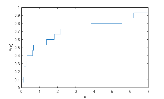
The figure shows that the cdf makes a large increase for small values of x and reaches 1 when x is near 7.