GPU を使用した相関の高速化
この例では、GPU を使用して相互相関を高速化する方法を示します。相関問題の多くは、大規模なデータセットを扱うことから、GPU の使用によりより高速な解決が可能です。この例では、Parallel Computing Toolbox™ のユーザー ライセンスが必要です。どの GPU がサポートされているかについては、GPU 計算の要件 (Parallel Computing Toolbox)を参照してください。
はじめに
まず、ご使用のマシンの GPU の基本的な情報を学習します。GPU にアクセスするには、Parallel Computing Toolbox を使用します。
if ~(parallel.gpu.GPUDevice.isAvailable)
    fprintf("\n\t**GPU not available. Stopping.**\n");
    return;
else
    dev = gpuDevice;
    fprintf(...
    "GPU detected (%s, %d multiprocessors, Compute Capability %s)", ...
    dev.Name, dev.MultiprocessorCount, dev.ComputeCapability);
end
GPU detected (NVIDIA RTX A5000, 64 multiprocessors, Compute Capability 8.6)
ベンチマーク機能
CPU 用に書かれたコードは GPU に移植して実行できるため、1 つの関数を CPU と GPU の両方のベンチマークに利用できます。ただし、GPU 上のコードは CPU とは非同期に実行されるため、性能測定には特別な注意が必要です。ある関数の実行に要した時間を測定する前に、すべての GPU 処理が終了しているか、デバイス上で 'wait' メソッドを実行して確認します。この追加の呼び出しは、CPU の性能には影響を与えません。
この例では、3 つの異なるタイプの相互相関のベンチマークを行います。
単純な相互相関のベンチマーク
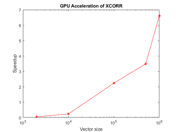
最初の例として、同じサイズの 2 つのベクトルが構文 xcorr(u,v) を使用して相互相関されています。GPU 実行時間に対する CPU 実行時間の比は、ベクトルのサイズに対してプロットされています。
sizes = floor(logspace(5,7,10))';
tc = zeros(numel(sizes),1);
tg = zeros(numel(sizes),1);

for s = 1:numel(sizes)
    if s == 1
        fprintf("** Benchmarking vector-vector cross-correlation. **")
        fprintf("Running xcorr of N elements")
    end
    fprintf(".");
    a = single(rand(sizes(s),1));
    b = single(rand(sizes(s),1));
    tc(s) = timeit(@() xcorr(a,b),1);
    tg(s) = gputimeit(@() xcorr(gpuArray(a),gpuArray(b)),1);
    if s == numel(sizes)
        disp(table(sizes,1e3*tc,1e3*tg,VariableNames= ...
            ["Length (N)" "CPU time (ms)" "GPU time (ms)"]))
    end
end
** Benchmarking vector-vector cross-correlation. **
Running xcorr of N elements
..........
    Length (N)    CPU time (ms)    GPU time (ms)
    __________    _____________    _____________

         1e+05       3.2248           1.1345
    1.6681e+05       6.0368           1.2935
    2.7826e+05       9.0778           1.5205
    4.6416e+05        16.32           1.9185
    7.7426e+05       25.602           2.5235
    1.2915e+06       56.349           3.7115
    2.1544e+06       85.022           7.5365
    3.5938e+06        143.4           13.051
    5.9948e+06       285.56           20.219
         1e+07       365.81           33.806
% Plot the results
fig = figure;
ax = axes(Parent=fig);
semilogx(ax,sizes,tc./tg,"r*-");
ylabel(ax,"Speedup");
xlabel(ax,"Vector size");
title(ax,"GPU Acceleration of XCORR");
行列の列の相互相関のベンチマーク
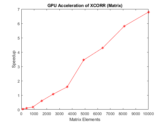
2 番目の例として、行列 A の列が、構文 xcorr(A) を使用して対相互相関され、すべての相関からなる大きな行列出力が生成されています。CPU の実行時間と GPU の実行時間の比率は、行列 A のサイズに対してプロットされています。
sizes = floor(logspace(2,2.5,10))';
tc = zeros(numel(sizes),1);
tg = zeros(numel(sizes),1);
for s = 1:numel(sizes)
    if s == 1
        fprintf("** Benchmarking matrix column cross-correlation. **")
        fprintf("Running xcorr (matrix) of an N-by-N matrix")
    end
    fprintf(".");
    a = single(rand(sizes(s)));
    tc(s) = timeit(@() xcorr(a),1);
    tg(s) = gputimeit(@() xcorr(gpuArray(a)),1);
    if s == numel(sizes)
        disp(table(sizes,1e3*tc,1e3*tg,VariableNames= ...
            ["Size (N)" "CPU time (ms)" "GPU time (ms)"]))
    end
end
** Benchmarking matrix column cross-correlation. **
Running xcorr (matrix) of an N-by-N matrix
..........
    Size (N)    CPU time (ms)    GPU time (ms)
    ________    _____________    _____________

      100          5.3818           0.80717
      113          8.0898           0.88967
      129          13.426            1.6885
      146          18.493            2.0345
      166            25.6            2.4435
      189          36.405            3.1765
      215          57.449            3.8975
      244          81.755            4.7185
      278          131.18            11.829
      316          178.32            15.023
% Plot the results
fig = figure;
ax = axes(Parent=fig);
semilogx(ax,sizes.^2,tc./tg,"r*-")
ylabel(ax,"Speedup")
xlabel(ax,"Matrix Elements")
title(ax,"GPU Acceleration of XCORR (Matrix)")
2 次元の相互相関のベンチマーク
最後の例として、X と Y の 2 つの行列が xcorr2(X,Y) を使用して相互相関されています。X のサイズは固定されており、Y のサイズは可変です。2 番目の行列のサイズに対する speedup の値がプロットされています。
sizes = floor(logspace(2.5,3.5,10))';
tc = zeros(numel(sizes),1);
tg = zeros(numel(sizes),1);
a = single(rand(100));

for s = 1:numel(sizes)
    if s == 1
        fprintf("** Benchmarking 2-D cross-correlation**")
        fprintf("Running xcorr2 of 100-by-100 and N-by-N matrices.")
    end
    fprintf(".");
    b = single(rand(sizes(s)));
    tc(s) = timeit(@() xcorr2(a,b),1);
    tg(s) = gputimeit(@() xcorr2(gpuArray(a),gpuArray(b)),1);
    if s == numel(sizes)
        disp(table(sizes,1e3*tc,1e3*tg,VariableNames= ...
            ["Size (N)" "CPU time (ms)" "GPU time (ms)"]))
    end
end
** Benchmarking 2-D cross-correlation**
Running xcorr2 of 100-by-100 and N-by-N matrices.
..........
    Size (N)    CPU time (ms)    GPU time (ms)
    ________    _____________    _____________

       316         3.9288           2.7275
       408         6.0308           2.9065
       527         9.4288           3.4885
       681         15.166           5.8805
       879         24.238           7.5805
      1136         37.586           12.254
      1467         65.472           18.775
      1895         109.37           28.703
      2448         171.28            42.79
      3162          299.2           70.185
% Plot the results
fig = figure;
ax =axes(Parent=fig);
semilogx(ax,sizes.^2,tc./tg,"r*-")
ylabel(ax,"Speedup")
xlabel(ax,"Matrix Elements")
title(ax,"GPU Acceleration of XCORR2")

GPU により高速化されたその他の信号処理関数
GPU 上で実行できるその他の信号処理関数がいくつかあります。これらの関数には、fft、ifft、conv、filter、fftfiltなどが含まれます。場合によっては、CPU に対しかなりの高速化が達成できます。GPU によって高速化された信号処理関数すべての一覧については、Signal Processing Toolbox™ ドキュメンテーションのGPU アルゴリズムの高速化の節を参照してください。
参考
gather (Parallel Computing Toolbox) | gpuArray (Parallel Computing Toolbox) | xcorr