メインコンテンツ

srs

R2026b

Shock response spectrum

Since R2026b

    Description

    S = srs(x,Fs) returns the Shock Response Spectrum (SRS) for the base acceleration signal x with a sample rate Fs Hz that stimulates an underdamped single-degree-of-freedom (SDOF) system.

    example

    S = srs(x,Ts) returns the SRS for the signal x that contains the base acceleration with a sample time Ts.

    S = srs(x) returns the SRS for the uniformly sampled MATLAB® timetable x that contains the base acceleration over time.

    example

    [S,Fn] = srs(___) returns the natural frequencies, Fn, associated with the SDOF system. You can specify input arguments as listed in any of the previous syntaxes.

    [S,Fn,infoSDOF] = srs(___) also returns information about the shock response in the time domain and the underlying SDOF system.

    example

    [___] = srs(___,Name=Value) specifies additional options using name-value arguments. You can specify the natural frequencies to use in the SDOF system, the quality factor, the type of shock response, among others.

    example

    srs(___) with no output arguments plots the SRS in the current figure window or specified target parent container.

    example

    Examples

    collapse all

    Generate and plot a rectangular-pulse acceleration signal with a width of 11 milliseconds, an amplitude of 0.33 m/s2, and a total duration of 30 milliseconds. The sample rate of the signal, Fs, is 100 kHz.

    Fs = 1e5; 
    tau = 11e-3; 
    tEnd = 30e-3; 
    t = (0:1/Fs:tEnd)'; 
    x = 0.33.*(t<=tau);
    
    plot(t,x)
    xlabel("Time (seconds)")
    ylabel("Acceleration (m/s^2)")
    grid on
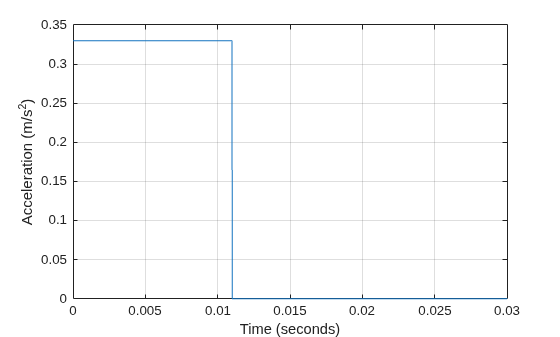
    Figure contains an axes object. The axes object with xlabel Time (seconds), ylabel Acceleration (m/s Squared baseline ) contains an object of type line.

    Calculate the SRS of the acceleration signal.

    S = srs(x,Fs);

    By default, the srs function associates S with a vector of natural frequencies, defined as an octave space from Fs/(3*2^15) to Fs/24 with six bands per octave. Use the default vector of natural frequencies to plot the SRS on a logarithmic scale.

    f = freqoctspace(Fs/(3*2^15),Fs/24,6, ...
        OctaveRatioBase=2,ReferenceFrequency=1);
    
    figure
    loglog(f,S,".")
    xlabel("Natural Frequency (Hz)")
    ylabel("Acceleration (m/s^2)")
    grid on
    ylim([0.01 1])
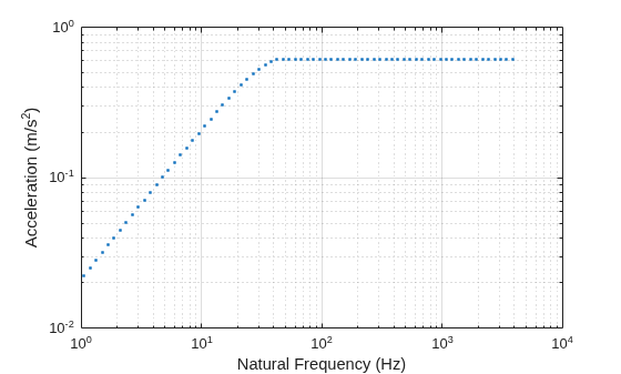
    Figure contains an axes object. The axes object with xlabel Natural Frequency (Hz), ylabel Acceleration (m/s Squared baseline ) contains a line object which displays its values using only markers.

    Generate a MATLAB® timetable containing a versed-sine acceleration signal with a width of 10 milliseconds and a total duration of 25 milliseconds. The sample rate of the shock signal is 100 kHz and the amplitude is 50 times the gravity acceleration on Earth.

    Fs = 1e5;
    A = 50*9.81;
    tau = 0.010;
    T = 0.025;
    t = (0:1/Fs:T)';
    vs = (A/2)*(1-cospi(2*t/tau)).*(t>=0 & t<=tau);
    
    vsTT = timetable(seconds(t),vs);

    Compute the SRS of the acceleration signal timetable.

    [S,Fn] = srs(vsTT);

    Plot the shock signal and the corresponding SRS.

    figure
    tiledlayout("vertical")
    nexttile
    plot(vsTT.Properties.RowTimes,vsTT{:,:})
    title("Shock Signal")
    xlabel("Time (s)")
    ylabel("Acceleration (m/s^2)")
    grid on
    nexttile
    loglog(Fn,S)
    title("Shock Response Spectrum")
    xlabel("Natural Frequency (Hz)")
    ylabel("Acceleration (m/s^2)")
    grid on
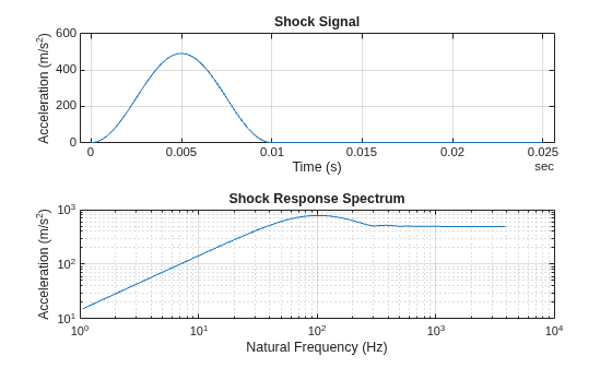
    Figure contains 2 axes objects. Axes object 1 with title Shock Signal, xlabel Time (s), ylabel Acceleration (m/s^2) contains an object of type line. Axes object 2 with title Shock Response Spectrum, xlabel Natural Frequency (Hz), ylabel Acceleration (m/s^2) contains an object of type line.

    Generate a vector containing a rectangular-pulse acceleration signal with a width of 7 milliseconds and a total duration of 10 milliseconds. The sample rate of the shock signal is 100 kHz and the amplitude is 10 times the gravity acceleration on Earth.

    tWidth = 0.007;
    tPulse = 0.01;
    Fs = 1e5;
    t = (0:1/Fs:tPulse)';
    x = 10*9.81*rectpuls(t,2*tWidth);

    Compute and plot the residual relative-acceleration SRS of the shock signal. Assume SDOF systems with a quality factor of 5. Plot a point on the SRS values at three natural frequencies.

    Q = 5;
    srsType = "relaccel";
    respSeg = "residual";
    [S,F,infoSDOF] = srs(x,Fs,QualityFactor=Q, ...
        ResponseType=srsType,ResponseSegment=respSeg,Parent=axes(figure));
    hold on
    FnIdx = [23 40 58];
    scatter(F(FnIdx),max(abs(infoSDOF.Responses(:,FnIdx))),"*")
    hold off
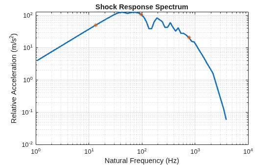
    Figure contains an axes object. The axes object with title Shock Response Spectrum, xlabel Natural Frequency (Hz), ylabel Relative Acceleration (m/s Squared baseline ) contains 2 objects of type line, scatter.

    From the SDOF information array, infoSDOF, extract and plot the shock responses corresponding to each SRS. Plot the shock signal along with the shock responses.

    • The residual shock responses measure the effects after the shock signal excites the SDOF.

    • The maximum absolute values of the residual shock responses are approximately 50, 110, and 20 m/s2 at the natural frequencies of 13.5 Hz, 95.9 Hz, and 767 Hz, respectively.

    figure
    for i = FnIdx
        plot(infoSDOF.Time,infoSDOF.Responses(:,i), ...
            DisplayName=sprintf("Shock Response (F_n =  %g Hz)",F(i)))
        hold on
    end
    plot(t,x,LineWidth=2,DisplayName="Input Shock")
    hold off
    xlim([0 0.1])
    xlabel("Time (s)")
    ylabel("Acceleration (m/s^2)")
    legend(Location="southeast")
    grid minor
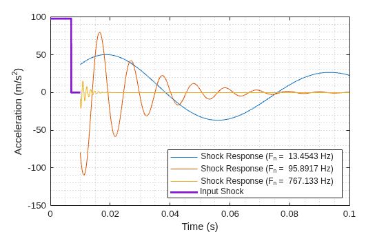
    Figure contains an axes object. The axes object with xlabel Time (s), ylabel Acceleration (m/s Squared baseline ) contains 4 objects of type line. These objects represent Shock Response (F_n = 13.4543 Hz), Shock Response (F_n = 95.8917 Hz), Shock Response (F_n = 767.133 Hz), Input Shock.

    Generate a half-sine acceleration signal with a width of 7 seconds, a delay of 2 seconds, and a total duration of 11 seconds. The sample rate of the shock signal is 2 kHz and the amplitude is 1 m/s2.

    tWidth = 7;
    tStart = 2;
    tPulse = 11;
    Fs = 2e3;
    
    t = (0:1/Fs:tPulse)';
    x = sinpi((t-tStart)/tWidth).*(t>=tStart & t<=(tStart+tWidth));

    Plot the primary and residual SRS of the shock signal using the maximum positive and maximum negative shock responses. Assume a SDOF system with natural frequencies linearly distributed from 0 Hz to 2 Hz and a damping ratio of 0.04.

    fn = linspace(0,2,201);
    Q = 1/(2*0.04);
    respSeg = ["primary" "residual"];
    peakType = ["maxpos" "maxneg"];
    
    ax = axes(figure);
    hold on
    for rs = respSeg
        for pt = peakType    
            srs(x,Fs,NaturalFrequency=fn,QualityFactor=Q, ...
                ResponseSegment=rs,PeakType=pt,Parent=ax)
        end
    end
    hold off
    lgnd = reshape(respSeg + ", "+ peakType',[],1);
    legend(lgnd)
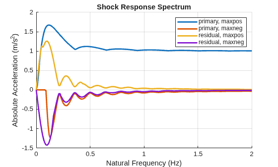
    Figure contains an axes object. The axes object with title Shock Response Spectrum, xlabel Natural Frequency (Hz), ylabel Absolute Acceleration (m/s Squared baseline ) contains 4 objects of type line. These objects represent primary, maxpos, primary, maxneg, residual, maxpos, residual, maxneg.

    This example plots the SRS for several half-sine shock signals with a sample rate of 5 kHz. Define SDOF systems with a quality factor of 25 and natural frequencies ranging linearly from 0.01 Hz to 500 Hz.

    Fs = 5e3;
    Q = 25;
    Fn = linspace(0.01,500,101);

    Plot the SRS of half-sine acceleration signals with a width of 10 milliseconds and amplitudes of 25, 50, and 100 m/s2. The absolute acceleration shown in each SRS is proportional to the amplitude of the corresponding half-sine acceleration signal.

    A = [25 50 100];
    W = 10*1e-3;
    tiledlayout(2,1)
    for a = A
        t = 0:1/Fs:W;
        x = a*sin(pi*t/W);
        ax = nexttile(1);
        hold on
        plot(1e3*t,x,LineWidth=2)
        nexttile(2)
        hold on
        srs(x,Fs,NaturalFrequency=Fn, ...
            QualityFactor=Q,RolloffMethod="none")
    end
    xlabel(ax,"Time (ms)")
    ylabel(ax,"Absolute Acceleration (m/s^2)")
    title(ax,"Shock Signal")
    axis(ax,[0 1.2e3*max(W) 0 max(A)])
    grid(ax,"on")
    lgn = legend(ax,"Amplitude: " + A + " m/s^2");
    title(lgn,"Width: " + 1e3*W + " ms")
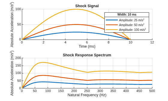
    Figure contains 2 axes objects. Axes object 1 with title Shock Signal, xlabel Time (ms), ylabel Absolute Acceleration (m/s^2) contains 3 objects of type line. These objects represent Amplitude: 25 m/s^2, Amplitude: 50 m/s^2, Amplitude: 100 m/s^2. Axes object 2 with title Shock Response Spectrum, xlabel Natural Frequency (Hz), ylabel Absolute Acceleration (m/s^2) contains 3 objects of type line.

    Plot the SRS of half-sine acceleration signals with an amplitude of width of 50 m/s2 and widths of 5, 10, and 20 milliseconds. The transient shown in each SRS is inversely proportional to the width of the corresponding half-sine acceleration signal.

    A = 50;
    W = [5 10 20]*1e-3;
    figure
    tiledlayout(2,1)
    for w = W
        t = 0:1/Fs:w;
        x = A*sin(pi*t/w);
        ax = nexttile(1);
        hold on
        plot(1e3*t,x,LineWidth=2)
        nexttile(2)
        hold on
        srs(x,Fs,NaturalFrequency=Fn, ...
            QualityFactor=Q,RolloffMethod="none")
    end
    xlabel(ax,"Time (ms)")
    ylabel(ax,"Absolute Acceleration (m/s^2)")
    title(ax,"Shock Signal")
    axis(ax,[0 1.2e3*max(W) 0 max(A)])
    grid(ax,"on")
    lgn = legend(ax,"Width: " + 1e3*W + " ms");
    title(lgn,"Amplitude: " + A + " m/s^2")
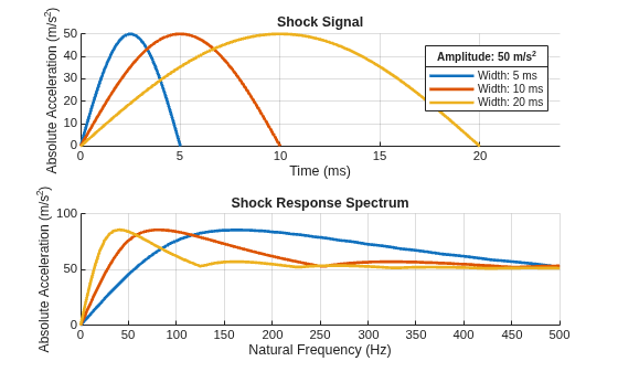
    Figure contains 2 axes objects. Axes object 1 with title Shock Signal, xlabel Time (ms), ylabel Absolute Acceleration (m/s^2) contains 3 objects of type line. These objects represent Width: 5 ms, Width: 10 ms, Width: 20 ms. Axes object 2 with title Shock Response Spectrum, xlabel Natural Frequency (Hz), ylabel Absolute Acceleration (m/s^2) contains 3 objects of type line.

    Generate a terminal-peak sawtooth acceleration signal with a width of 10 milliseconds. The sample rate of the shock signal is 20 kHz and the amplitude is 100 m/s2.

    Fs = 20e3;
    A = 100;
    W = 0.01;
    tps = A*(0:1/Fs:W)/W;

    When a SDOF system has a damping ratio of zero (infinite quality factor), the pseudo velocity spectrum at low frequency (close to 0 Hz) tends toward the area under the shock pulse. For a terminal-peak sawtooth shock waveform with amplitude A and width W, the area is A×W/2.

    area = sum(tps)/Fs
    area = 
    0.5025
    

    Compute and plot the pseudo-velocity SRS of the acceleration signal. Assume SDOF systems with an infinite quality factor and natural frequencies ranging in an octave space from 0.01 Hz to 1 kHz with 12 intervals per octave.

    fn = freqoctspace(0.01,1e3,12);
    Q = Inf;
    
    fig = figure;
    ax = axes(fig);
    srspec = srs(tps,Fs,NaturalFrequency=fn,QualityFactor=Q, ...
        ResponseType="pseudovel",Parent=ax);
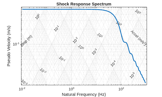
    Figure contains an axes object. The axes object with title Shock Response Spectrum, xlabel Natural Frequency (Hz), ylabel Pseudo Velocity (m/s) contains 133 objects of type text, line.

    Display the pseudo velocity SRS value at the lowest natural frequency and compare it with the area under the shock pulse.

    fprintf("Area under shock = %.4f\n" + ...
        "Pseudovelocity at low frequency = %.4f\n",area,srspec(1))
    Area under shock = 0.5025
    Pseudovelocity at low frequency = 0.5025
    

    Input Arguments

    collapse all

    Base acceleration signal in m/s2, specified as a real-valued vector, matrix, or timetable.

    This argument represents the base acceleration in m/s2 that stimulates an underdamped SDOF oscillator.

    • The signal must have at least nine elements if x is a vector, or nine rows if x is a matrix or a timetable.

    • All the elements in x must be finite.

    • If you specify x as a matrix, then the srs function interprets its columns as individual channels.

    • If you specify x as a timetable:

      • x must be uniformly sampled.

      • x can have one variable with multiple channels, or multiple variables with one channel each.

      Only timetables that use a duration or datetime vector for RowTimes are supported.

    Example: x = randn(5000,12) specifies a random with 5000 samples and 12 channels. To specify the sample rate or sample time,use Fs.

    Example: x = timetable(randn(5000,12),SampleRate=1e3) specifies a 12-channel random variable sampled at 1 kHz for 5 seconds.

    Data Types: single | double

    Sample rate, specified as a numeric scalar.

    • The function uses the value specified in this argument to calculate the times associated with the vector or matrix x.

    • This argument does not apply if x is a timetable.

    Data Types: single | double

    Sample time, specified as a duration scalar.

    • The function uses the value specified in this argument to calculate the sample rate and the times associated with the vector or matrix x.

    • This argument does not apply if x is a timetable

    Data Types: duration

    Name-Value Arguments

    collapse all

    Specify optional pairs of arguments as Name1=Value1,...,NameN=ValueN, where Name is the argument name and Value is the corresponding value. Name-value arguments must appear after other arguments, but the order of the pairs does not matter.

    Example: [S,Fn] = srs(rand(1000,1),2e3,QualityFactor=7,ResponseType="relvel") computes the relative-velocity SRS of a 1000-sample base acceleration signal sampled at a rate of 2 kHz, where the underlying SDOF uses a quality factor of 7.

    Natural frequencies in Hz, specified as a vector of nonnegative values less than or equal to the Nyquist rate.

    By default, the srs function uses the sample rate Fs to generate the natural frequencies as a logarithmically spaced vector from Fs/(3*2^15) to Fs/24 with a space of one sixth of octave.

    • The function uses the minimum natural frequency of Fs/(3*2^15) to ensure sufficient frequency resolution to accurately estimate low-frequency SDOF responses.

    • The function uses the maximum natural frequency of Fs/24 to aim a peak estimation error under 1% at high frequencies.

    • The function uses the 1/6 octave spacing between natural frequencies to follow the MIL-STD-810H standard [1], and offers a practical balance between frequency resolution and statistical independence across shock response spectrum estimates.

    • To generate frequency vector with octave spacing, you can use the freqoctspace function. Given the sample rate Fs, this code generates the default 72-element vector of natural frequencies, NFreqs, if you do not specify NaturalFrequency.

      NFreqs = freqoctspace(Fs/(3*2^15),Fs/24,6,OctaveRatioBase=2,ReferenceFrequency=1);

      You can alternatively use the logspace function to generate a logarithmically spaced vector of natural frequencies.

    Data Types: single | double

    Quality factor, specified as positive scalar greater than 0.5.

    The quality factor Q and the damping ratio ζ of the underlying SDOF system are related by Q = (2ζ)–1.

    • The SDOF system must be underdamped (ζ < 1), thus Q must be greater than 0.5.

    • The default value for this argument (Q = 10) considers a 5% damping ratio (ζ = 0.05).

    Data Types: single | double

    Type of shock response, specified as one of these values:

    • "absaccel" — Absolute acceleration

    • "relaccel" — Relative acceleration

    • "pseudoaccel" — Pseudo acceleration, defined as ξ·ω2n, where:

      • ξ is the relative displacement.

      • ωn is the natural angular frequency.

    • "relvel" — Relative velocity

    • "pseudovel" — Pseudo velocity, defined as ξ·ωn.

    • "reldisp" — Relative displacement

    The function computes the SRS based on the type of shock response specified in this argument.

    Data Types: char | string

    Segment of the shock response from which to compute the SRS, specified as one of these values:

    • "full" — Use the time range associated with the input x and the post-input response.

    • "primary" — Use the time range associated with the input only.

    • "residual" — Use the time range associated with the post-input response only.

    The function computes the SRS using the peak response at the times corresponding to the type of time range specified in this argument.

    If you specify this argument as "full" or "residual", then the function pads the input signal with zeros for the time range associated with the post-input response.

    • The number of padded zeros equals the duration of one period at the lowest natural frequency. For a vector of natural frequencies NFreqs specified in NaturalFrequency and a sample rate Fs, the number of padded zeros equals ceil(Fs/min(NFreqs)).

    • If NaturalFrequency contains a 0 Hz frequency, then the function does not perform zero padding.

    Data Types: char | string

    Length of the shock signal, specified as a positive integer (number of samples) or as a duration scalar (time in seconds).

    The shock signal defines the time window over which the primary excitation is assumed to occur.

    • The value specified in this argument cannot exceed the total length or duration of the input signal x.

    • You can specify this argument only if you specify ResponseSegment as "primary" or "residual".

    • If you specify ShockLength as a duration scalar, the specified value must be at least seconds(1/Fs) or Ts, so that the length of the shock signal spans at least one sample.

    Data Types: single | double

    Method to extract the peak response, specified as "maximax", "maxneg", ."maxpos", or "rms".

    Assume a shock response s, which is the response of a SDOF to the input x, then the function extracts the peak response p depending on the value specified in this argument:

    • "maximax" — srs finds the absolute maximum peak, p = max(abs(s)).

    • "maxneg" — srs finds the maximum value in the negative direction, p = min(s).

    • "maxpos" — srs finds the maximum value in the positive direction, p = max(s).

    • "rms" — srs computes the root-mean-square of the shock response, p = rms(s).

    Data Types: char | string

    Method to preprocess the base acceleration signal x, specified as one of these values:

    • "prefilter" — srs filters x using a zero-phase third-order filter with a high-frequency gain. The function uses this method to compensate for the attenuation that the ramp-invariant transformation introduces. For more information, see Algorithms.

    • "resample" — srs resamples x using an FIR antialiasing lowpass filter.

      The function uses this method to enforce the points-per-cycle requirement that you specify in PointsPerCycle.

    • "interp" — srs linearly interpolates x using shape-preserving piecewise cubic polynomials.

      The function uses this method to enforce the points-per-cycle requirement that you specify in PointsPerCycle.

    • "none" — srs does not preprocess x.

    The function then uses the preprocessed base acceleration signal to compute the shock response.

    Data Types: char | string

    Minimum number of points per cycle to compute the shock response, specified as a positive integer.

    Assume a vector of natural frequencies specified as NaturalFrequency=NFreqs, a sample rate Fs, and the minimum number of points per cycle specified as PointsPerCycle=Nppc.

    • If max(NFreqs)/Fs < Nppc, then the function interpolates or resamples the base acceleration signal x to satisfy the required number of points per cycle.

    • Lower values of Nppc decrease the computation accuracy while higher values of Nppc increase the computation time.

    • The maximum peak error is emax = 1 – cos(π/Nppc), so the default value Nppc = 12 corresponds to emax = 0.034 (3.4%).

    This argument applies only if you specify RolloffMethod as "resample" or "interp".

    Data Types: single | double

    Target parent container, specified as an Axes object, a UIAxes object, or a Panel object.

    If you specify Parent, the srs function plots the SRS on the specified target parent container, whether you call the function with or without output arguments.

    For more information about target containers and the parent-child relationship in MATLAB graphics, see Graphics Object Hierarchy. For more information about using Parent in UIAxes and Panel objects to design apps, see Plot Spectral Representations of Signal in App Designer.

    Output Arguments

    collapse all

    Shock response spectrum (SRS), returned as a column vector or a matrix with as many columns as x.

    Natural frequencies, returned as a column vector with as many rows as S.

    If you specify NaturalFrequency, then the function returns the specified vector in Fn.

    SRS information, returned as a struct array that comprises the following fields:

    • Time — Times associated with the shock response, returned as a column vector.

      The function does not return Time if x is a timetable. Instead, the function returns Responses as a timetable with the corresponding time information.

    • Responses — Shock responses in the time domain, returned as one of these:

      • Matrix with as many columns as natural frequencies — Each column corresponds to a natural frequency.

      • 3-D array with as many pages as natural frequencies — Each column corresponds to a channel or column of x, while each page corresponds to a natural frequency.

      • Timetable — Each variable is a 3-D array where each row corresponds to a time instance, each column corresponds to a channel or column of x, while each page corresponds to a natural frequency.

    • Systems — SDOF system information, returned as a struct array that comprises these fields:

      • Numerator — Numerator coefficients of the SDOF system, returned as a matrix with as many rows as natural frequencies. The ith column corresponds to the z–(i-1) term.

      • Denominator — Denominator coefficients of the SDOF system, returned as a matrix with as many rows as natural frequencies. The ith column corresponds to the z–(i-1) term.

      • IsStable — SDOF stability status at each natural frequency, returned as a column vector.

        To determine stability, srs uses the isstable function and the Coefficients field. For the natural frequencies at which the SDOF system is unstable, the function returns 0 in the corresponding rows of IsStable. At these frequencies, the computed SRS might be inaccurate.

    More About

    collapse all

    Algorithms

    By default (if you set RolloffMethod to "prefilter"), the srs function uses the prefilter-Smallwood method [5], which uses ramp invariance to convert the transfer function to an equivalent digital filter with unit DC response.

    • In this case, srs uses filtfilt to zero-phase filter x for ramp invariance, and then uses Smallwood's method [6] to compute the SRS of x.

    • Aliasing is the main reason that the digital filter obtained from the impulse-invariant method does not have a unit DC response. Thus, ramp invariance connects impulse-response samples with straight lines to decrease aliasing.

    If you set RolloffMethod to "none", then srs does not perform zero-phase filtering and uses Smallwood's method to compute the SRS of x.

    References

    [1] Environmental Engineering Considerations and Laboratory Tests — Test Method Standard (2019). MIL-STD-810H. Melville, NY: US Department of Defense.

    [2] Lalanne, C. (2009) Mechanical Vibration and Shock Analysis. Vol. 2: Mechanical Shock / Christian Lalanne. Second edition, London: ISTE.

    [3] Piersol, A. G., Paez, T. L., and Harris, C M. (2010) Harris’ Shock and Vibration Handbook. 6th ed. New York: McGraw-Hill.

    [4] Kelly, R. D., and Richman, G. (1969) Principles and Techniques of Shock Data Analysis. Washington: Naval Research Laboratory.

    [5] Ahlin, K. (1999) "Shock Response Spectrum Calculation - An Improvement of the Smallwood Algorithm." 70th Shock and Vibration Symposium. SAVIAC.

    [6] Smallwood, D. O. “Improved Recursive Formula for Calculating Shock Response Spectra.” (1980) Shock and Vibration Bulletin, Vol. 51, Number 2, pp. 211–17.

    Extended Capabilities

    expand all

    C/C++ Code Generation
    Generate C and C++ code using MATLAB® Coder™.

    GPU Code Generation
    Generate CUDA® code for NVIDIA® GPUs using GPU Coder™.

    Version History

    Introduced in R2026b