derivative

Time derivative of manipulator model states

Since R2019b

Syntax

stateDot = derivative(taskMotionModel,state,refPose,refVel)

stateDot = derivative(taskMotionModel,state,refPose, refVel,fExt)

stateDot = derivative(jointMotionModel,state,cmds)

stateDot = derivative(jointMotionModel,state,cmds,fExt)

Description

stateDot = derivative(taskMotionModel,state,refPose,refVel) computes the time derivative of the motion model based on the current state and motion commands using a task-space model.

stateDot = derivative(taskMotionModel,state,refPose, refVel,fExt) computes the time derivative based on the current state, motion commands, and any external forces on the manipulator using a task space model.

stateDot = derivative(jointMotionModel,state,cmds) computes the time derivative of the motion model based on the current state and motion commands using a joint-space model.

stateDot = derivative(jointMotionModel,state,cmds,fExt) computes the time derivative based on the current state, motion commands, and any external forces on the manipulator using a joint-space model.

Examples

Create Joint-Space Motion Model

This example shows how to create and use a jointSpaceMotionModel object for a manipulator robot in joint-space.

Create the Robot

robot = loadrobot("kinovaGen3","DataFormat","column","Gravity",[0 0 -9.81]);

Set Up the Simulation

Set the timespan to be 1 s with a timestep size of 0.01 s. Set the initial state to be the robots, home configuration with a velocity of zero.

tspan = 0:0.01:1;
initialState = [homeConfiguration(robot); zeros(7,1)];

Define the a reference state with a target position, zero velocity, and zero acceleration.

targetState = [pi/4; pi/3; pi/2; -pi/3; pi/4; -pi/4; 3*pi/4; zeros(7,1); zeros(7,1)];

Create the Motion Model

Model the system with computed torque control and error dynamics defined by a moderately fast step response with 5% overshoot.

motionModel = jointSpaceMotionModel("RigidBodyTree",robot);
updateErrorDynamicsFromStep(motionModel,.3,.05);

Simulate the Robot

Use the derivative function of the model as the input to the ode45 solver to simulate the behavior over 1 second.

[t,robotState] = ode45(@(t,state)derivative(motionModel,state,targetState),tspan,initialState);

Plot the Response

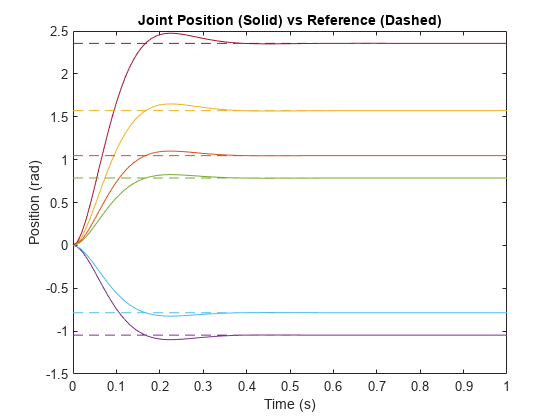
Plot the positions of all the joints actuating to their target state. Joints with a higher displacement between the starting position and the target position actuate to the target at a faster rate than those with a lower displacement. This leads to an overshoot, but all of the joints have the same settling time.

figure
plot(t,robotState(:,1:motionModel.NumJoints));
hold all;
plot(t,targetState(1:motionModel.NumJoints)*ones(1,length(t)),"--");
title("Joint Position (Solid) vs Reference (Dashed)");
xlabel("Time (s)")
ylabel("Position (rad)");

Create Task-Space Motion Model

This example shows how to create and use a taskSpaceMotionModel object for a manipulator robot arm in task-space.

Create the Robot

robot = loadrobot("kinovaGen3","DataFormat","column","Gravity",[0 0 -9.81]);

Set Up the Simulation

Set the time span to be 1 second with a timestep size of 0.02 seconds. Set the initial state to the home configuration of the robot, with a velocity of zero.

tspan = 0:0.02:1;
initialState = [homeConfiguration(robot);zeros(7,1)];

Define a reference state with a target position and zero velocity.

refPose = trvec2tform([0.6 -.1 0.5]);
refVel = zeros(6,1);

Create the Motion Model

Model the behavior as a system under proportional-derivative (PD) control.

motionModel = taskSpaceMotionModel("RigidBodyTree",robot,"EndEffectorName","EndEffector_Link");

Simulate the Robot

Simulate the behavior over 1 second using a stiff solver to more efficiently capture the robot dynamics. Using ode15s enables higher precision around the areas with a high rate of change.

[t,robotState] = ode15s(@(t,state)derivative(motionModel,state,refPose,refVel),tspan,initialState);

Plot the Response

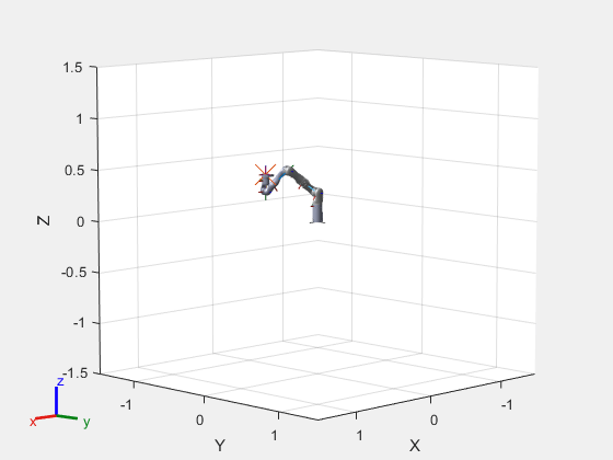
Plot the robot's initial position and mark the target with an X.

figure
show(robot,initialState(1:7));
hold all
plot3(refPose(1,4),refPose(2,4),refPose(3,4),"x","MarkerSize",20)

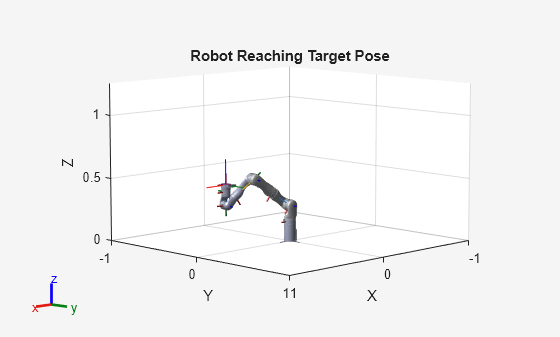
Observe the response by plotting the robot in a 5 Hz loop.

r = rateControl(5);
for i = 1:size(robotState,1)
    show(robot,robotState(i,1:7)',"PreservePlot",false);
    waitfor(r);
end

Input Arguments

taskMotionModel — taskSpaceMotionModel object

taskSpaceMotionModel object

taskSpaceMotionModel object, which defines the properties of the motion model.

jointMotionModel — jointSpaceMotionModel object

jointSpaceMotionModel object

jointSpaceMotionModel object, which defines the properties of the motion model.

state — Joint positions and velocities

1-by-2n-element vector

Joint positions and velocities represented as a 2n-element vector, specified as [q; qDot]. n is the number of non-fixed joints in the associated rigidBodyTree of the motionModel. q, represents the position of each joint, specified in radians. qDot represents the velocity of each joint, specified in radians per second.

refPose — Robot pose

4-by-4 matrix

The reference pose of the end effector in the task-space in meters, specified as an 4-by-4 homogeneous transformation matrix.

refVel — Joint velocities

six-element row vector

The reference velocities of the end effector in the task space, specified as a six-element vector of real values, specified as [omega v]. omega represents a row vector of three angular velocities about the x, y, and z axes, specified in radians per second, and v represents a row vector of three linear velocities along the x, y, and z axes, specified in meters per second.

cmds — Control commands indicating desired motion

2-by-n matrix | 3-by-n matrix

Control commands indicating desired motion. The dimensions of cmds depend on the MotionType property of the motion model:

• "PDControl" — 2-by-n matrix, [qRef; qRefDot]. The first and second rows represent joint positions and joint velocities, respectively.

• "ComputedTorqueControl" — 3-by-n matrix, [qRef; qRefDot; qRefDDot]. The first, second, and third rows represent joint positions, joint velocities, and joint accelerations respectively.

• "IndependentJointMotion" — 3-by-n matrix, [qRef; qRefDot; qRefDDot]. The first, second, and third rows represent joint positions, joint velocities, and joint accelerations respectively.

Note that jointSpaceMotionModel supports all three MotionType listed above, but taskSpaceMotionModel only supports "PDControl" MotionType.

fExt — Joint positions and velocities

m-element vector

External forces, specified as an m-element vector, where m is the number of bodies in the associated rigidBodyTree object.

Output Arguments

stateDot — Time derivative of current state

2-by-n matrix

Time derivative based on current state and specified control commands, returned as a 2-by-n matrix of real values, [qDot; qDDot], where qDot is an n-element row vector of joint velocities, and qDDot is an n-element row vector of joint accelerations. n is the number of joints in the associated rigidBodyTree of the motionModel.

Extended Capabilities

C/C++ Code Generation
Generate C and C++ code using MATLAB® Coder™.

Version History

Introduced in R2019b