Custom Training Loop with Simulink Action Noise
This example shows how to tune a controller for vehicle platooning applications using a custom reinforcement learning (RL) training loop. For this application, action noise is generated in the Simulink® model to promote exploration during training.
For an example on tuning a PID-based vehicle platooning system, see Design Controller for Vehicle Platooning (Simulink Control Design).

Platooning has the following control objectives [1].
Individual vehicle stability — Spacing error for each following vehicle converges to zero if the preceding vehicle is traveling at constant speed.
String stability — Spacing errors do not amplify as they propagate toward the tail of the vehicle string.
Platooning Environment Model
In this example, there are five vehicles in the platoon. Every vehicle is modeled as a truck-trailer system with the following parameters. All lengths are in meters.
L1 = 6;               % Truck length
L2 = 10;              % Trailer length
M1 = 1;               % Hitch length
L = L1 + L2 + M1 + 5; % Desired front-to-front vehicle spacing
The lead vehicle follows a given acceleration profile. Each trailing vehicle has a controller that controls its acceleration.
Open the Simulink® model.
mdl = "fiveVehiclePlatoonEnv";
open_system(mdl)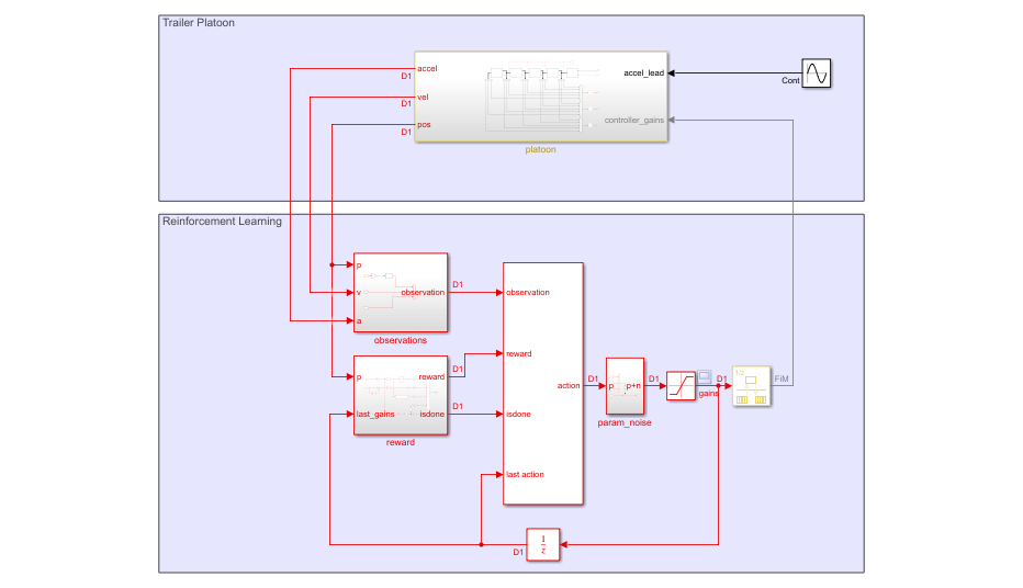
The model contains an RL Agent block with its last action input port enabled. This input port allows the specification of custom noise in the Simulink model for off-policy RL agents, such as deep deterministic policy gradient (DDPG) agents.
Specify the path to the RL Agent block.
agentBlk = mdl + "/RL Agent";Controller Structure
In this example, each trailing vehicle (ego vehicle) has the same continuous-time controller structure and parameterization.
Here:
, , and are the respective acceleration, velocity, and position of the ego vehicle.
, , and are the respective acceleration, velocity, and position of the vehicle directly in front of the ego vehicle.
Each vehicle has full access to its own velocity and position states but can only access the acceleration, velocity, and position of the vehicle directly in front using wireless communication.
The controller minimizes the velocity error using the velocity gain and minimizes the spacing error using the spacing gain . The feedforward gain is used to improve tracking of the front vehicle.
The lead vehicle' acceleration is assumed to be a sine wave
Here:
is the lead vehicle acceleration (m/s^2).
is the amplitude of the sine wave (m/s).
is the frequency of the sine wave (rad/s).
is the current simulation time (s).
Reinforcement Learning Agent Design
The objective of the agent is to compute adaptive gains so that each vehicle can track the desired spacing with respect to the vehicle immediately in front. Therefore, the model is configured such that:
The action signal consists of the gains shared by all vehicles except the lead vehicle. Each gain has a lower bound of 0 and upper bounds of 1, 20, and 20, respectively. The agent calculates new gains once per second. To encourage exploration during training, the gains are perturbed by random noise with a zero-mean normal distribution: where the variance .
The observation signal consists of the vehicle spacing ( minus the target spacing (, the vehicle velocities (), and the vehicle accelerations ().
The reward calculated at every time step is
where:
is the vehicle spacing () at time step .
calculates the max overshoot of all vehicles given the actual vehicle spacing and the desired spacing . In this case, overshoot is defined as when the vehicle spacing is less than the desired spacing .
indicates if a vehicle collision occurs. The simulation will terminate if is true.
The first term in the reward function encourages the vehicle spacing to match . The second term penalizes large changes in gain between time steps. The third term penalizes overshooting the target spacing (getting too close to the front vehicle). Finally, the fourth term penalizes collisions.
For this example, to accommodate the custom noise specified in the model, you implement a custom DDPG training loop.
Define Model Parameters
Define the training and simulation parameters that remain fixed during training.
Ts = 1;                       % Sample time (seconds)
Tf = 100;                     % Simulation length (seconds)
AccelNoiseV = ones(1,5)*0.01; % Acceleration input noise variance
VelNoiseV = ones(1,5)*0.01;   % Velocity sensor noise variance
PosNoiseV = ones(1,5)*0.01;   % Position sensor noise variance
ParamLowerLimit = [0 0 0]';   % Lower limits for the controller gains
ParamUpperLimit = [1 20 20]'; % Upper limits for the controller gains
UseParamNoise = 1;            % Option to indicate noise injection
Define the parameters that change every training episode. The values for these parameters are updated in the environment reset function resetFunction.
LeadA = 2;                    % Lead vehicle acceleration amplitude
LeadF = 1;                    % Lead vehicle acceleration frequency
ParamNoiseV = [0.02 0.1 0.1]; % Variance for controller gains

% Random noise seeds
ParamNoiseSeed = 1:3;       % Controller gain noise seed
AccelNoiseSeed = 1:5 + 100; % Acceleration input noise seed
VelNoiseSeed = 1:5 + 200;   % Velocity sensor noise seed
PosNoiseSeed = 1:5 + 300;   % Position sensor noise seed

% Initial position and velocity of each vehicle
InitialPositions  = [200 150 100 50 0] + 50; % Positions
InitialVelocities = [10 10 10 10 10];        % Velocities
Create Environment
Create an environment using rlSimulinkEnv.
To do so, first define the observation and action specifications for the environment.
obsInfo = rlNumericSpec([14 1]);
actInfo = rlNumericSpec([3  1], ...
    LowerLimit=ParamLowerLimit, ...
    UpperLimit=ParamUpperLimit);

obsInfo.Name = "measurements";
actInfo.Name = "control_gains";
Next, create the environment object.
env = rlSimulinkEnv(mdl,agentBlk,obsInfo,actInfo);
Set the environment reset function to the local function resetFunction included with this example. This function varies the training conditions for each episode.
env.ResetFcn = @resetFunction;
Noise in the model is specified using the Random Number (Simulink) block. Each block has its own random number generator and thus its own starting seed parameter. To ensure the noise stream varies across episodes, the seed variables are updated using resetFunction.
Create Actor, Critic, and Policy
Create actor and critic function approximators for the agent using the local function createNetworks included with this example.
[critic,actor] = createNetworks(obsInfo,actInfo);
Create optimizer objects for updating the actor and critic. Use the same options object for both optimizers. For more information, see rlOptimizerOptions and rlOptimizer.
optimizerOpt = rlOptimizerOptions( ...
    LearnRate=1e-3, ...
    GradientThreshold=1, ...
    L2RegularizationFactor=1e-2);
criticOptimizer = rlOptimizer(optimizerOpt);
actorOptimizer  = rlOptimizer(optimizerOpt);
Create a deterministic policy for the actor approximator. For more information, see rlDeterministicActorPolicy.
policy = rlDeterministicActorPolicy(actor);
Specify the policy sample time.
policy.SampleTime = Ts;
Create Experience Buffer
Create an experience buffer for the agent with a maximum length of 1e6.
replayMemory = rlReplayMemory(obsInfo,actInfo,1e6);
Data Required for Learning
To update the actor and critic during training, the runEpisode function calls a processing function to process each experience as it is received from the environment. For this example, the processing function is the local function processExperienceFcn.
This function requires additional data to perform its processing. Create a structure to store this additional data.
processExpData.Critic = critic;
processExpData.TargetCritic = critic;
processExpData.Actor = actor;
processExpData.TargetActor = actor;
processExpData.ReplayMemory = replayMemory;
processExpData.CriticOptimizer = criticOptimizer;
processExpData.ActorOptimizer = actorOptimizer;

processExpData.MiniBatchSize = 128;
processExpData.DiscountFactor = 0.99;
processExpData.TargetSmoothFactor = 1e-3;

% provide accelerated functions to processExpData
% to accelerate gradient computations

processExpData.AccelCriticGradFcn = ...
    dlaccelerate(@deepCriticGradient);

processExpData.AccelActorGradFcn  = ...
    dlaccelerate(@deepActorGradient);
During each episode, the processExperienceFcn function updates the critics, actors, replay memory, and optimizers. The updated data is used as the input for the next episode.
Training Loop
To train the agent, the custom training loop simulates the agent in the environment for a maximum of maxEpisodes episodes.
maxEpisodes = 1000;
Compute the maximum number of steps per episode using the simulation time and sample time.
maxSteps = ceil(Tf/Ts);
For this custom training loop:
The
runEpisodefunction simulates the agent in the environment for one episode.Experiences are processed as they are received from the environment using the
processExperienceFcnfunction.Experiences are not logged by
runEpisodesince they are processed as they are received.To speed up training, when calling
runEpisode, theCleanupPostSimoption is set tofalse. Doing so keeps the model compiled between episodes.The
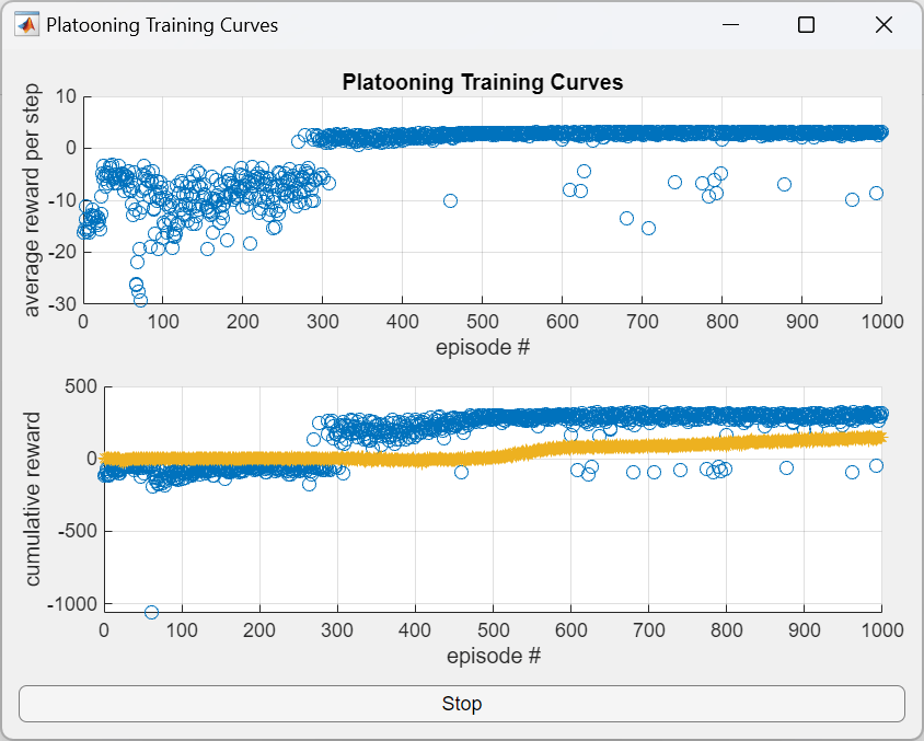
PlatooningTrainingCurvePlotterobject is a helper object to plot training data while the training is running.You can stop the training using a Stop button in the training plot.
After all the episodes are complete, the
cleanupfunction cleans up the environment and terminates the model compilation.
Training the policy is a computationally intensive process that can take several minutes to hours to complete. To save time while running this example, load a pretrained agent by setting doTraining to false. To train the policy yourself, set doTraining to true.
doTraining = false;
if doTraining
    % Create plotting helper object.
    plotObj = PlatooningTrainingCurvePlotter();

    % Training loop
    for i = 1:maxEpisodes

        % Run the episode.
        out = runEpisode( ...
            env,policy, ...
            MaxSteps=maxSteps, ...
            ProcessExperienceFcn=@processExperienceFcn, ...
            ProcessExperienceData=processExpData, ...
            LogExperiences=false, ...
            CleanupPostSim=false);

        % Extract episode information
        % to update the training curves.
        episodeInfo = out.AgentData.EpisodeInfo;

        % Extract updated processExpData for the next episode.
        processExpData = out.AgentData.ProcessExperienceData;
        % Extract the updated policy for the next episode.
        policy = out.AgentData.Agent;

        % Extract critic and actor approximators
        % from processExpData.
        critic = processExpData.Critic;
        actor  = processExpData.Actor;

        % Extract the cumulative reward and calculate
        % average reward per step for this episode.
        cumulativeRwd = episodeInfo.CumulativeReward;
        avgRwdPerStep = cumulativeRwd/episodeInfo.StepsTaken;

        % Evaluate q0 from the initial episode observation.
        obs0 = episodeInfo.InitialObservation;
        q0 = evaluate(critic,[obs0,evaluate(actor,obs0)]);
        q0 = double(q0{1});

        % Update the plot.
        update(plotObj,i,avgRwdPerStep,cumulativeRwd,q0);

        % Exit training if button pushed.
        if plotObj.StopTraining
            break;
        end
    end

    % Clean up the environment.
    cleanup(env);

    % Save the policy.
    save("PlatooningDDPGPolicy.mat","policy");
else
    % Load the pretrained policy.
    load("PlatooningDDPGPolicy.mat");
end
Validate Trained Policy
Validate the learned policy by running five simulations with random initial conditions specified by the reset function.
First, turn off parameter noise in the model.
UseParamNoise = 0;
Simulate the model against the trained policy five times.
N = 5;
simOpts = rlSimulationOptions( ...
    MaxSteps=maxSteps, ...
    NumSimulations=N);
experiences = sim(env,policy,simOpts);
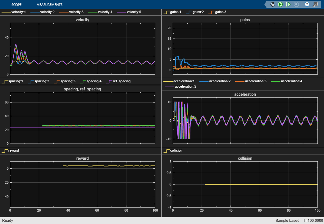
Plot the vehicle spacing error, gains, and reward from the experiences output structure.
f = figure(Position=[100 100 1024 768]);
tiledlayout(f,N,3);
for i = 1:N

    % Get the spacing.
    tspacing = experiences(i).Observation.measurements.Time;
    spacing  = ...
    squeeze(experiences(i).Observation.measurements.Data(1:4,:,:));

    % Get the gains.
    tgains = experiences(i).Action.control_gains.Time;
    gains  = squeeze(experiences(i).Action.control_gains.Data);

    % Get the reward.
    trwd = experiences(i).Reward.Time;
    rwd  = experiences(i).Reward.Data;

    % Plot the spacing.
    nexttile
    stairs(tspacing,spacing');
    title(sprintf("Vehicle Spacing Error Simulation %u",i))
    grid on

    % plot the gains.
    nexttile
    stairs(tgains,gains');
    title(sprintf("Vehicle Gains Simulation %u",i))
    grid on

    % Plot the reward.
    nexttile
    stairs(trwd,rwd);
    title(sprintf("Vehicle Reward Simulation %u",i))
    grid on
end

From the plots, you can see that the trained policy generates adaptive gains that adequately track the desired spacing for all vehicles.
Local Functions
The process experience function is called every time an experience is processed by the RL Agent block. Here, processExperienceFcn appends the experience to the replay memory, samples a mini-batch of experiences from the replay memory, and updates the critic, actor, and target networks.
function [policy,procExpData] = processExperienceFcn( ...
    exp,episodeInfo,policy,procExpData)

% Append experience to replay memory buffer.
append(procExpData.ReplayMemory,exp);

% Sample a mini-batch of experiences from replay memory.
% Return the mini-batch elements as dlarray objects so
% they can be treated as input to the automatically
% differentiated loss functions.
miniBatch = sample(procExpData.ReplayMemory, ...
    procExpData.MiniBatchSize, ...
    DiscountFactor=procExpData.DiscountFactor, ...
    ReturnDlarray=true);

if ~isempty(miniBatch)
    % Update network parameters using the mini-batch.
    procExpData = learnFcn(procExpData,miniBatch);

    % Update the policy parameters using the actor parameters.
    policy = setLearnableParameters( ...
        policy, ...
        getLearnableParameters(procExpData.Actor) ...
        );
end

end
The learnFcn function uses syncParameters to update the critic, actor, and target networks given a sampled mini-batch.
function processExpData = learnFcn(processExpData,miniBatch)

% Compute target next actions against the next observations.
nextAction = getAction( ...
    processExpData.TargetActor,miniBatch.NextObservation);

% compute qtarget = reward + gamma*Q(nextObservation,nextAction)
%                 = reward + gamma*expectedFutureReturn
% Bootstrap the target at non-terminal experiences.
gamma = processExpData.DiscountFactor.*single(miniBatch.IsDone~=1);
expectedFutureReturn = getValue(processExpData.TargetCritic, ...
    miniBatch.NextObservation,nextAction);
targetq = miniBatch.Reward + gamma.*expectedFutureReturn;

% Compute critic gradient using deepCriticGradient function.
criticGradient = dlfeval( ...
    processExpData.AccelCriticGradFcn, ...
    processExpData.Critic, ...
    miniBatch.Observation, ...
    miniBatch.Action,targetq);

% Update the critic parameters.
[processExpData.Critic,processExpData.CriticOptimizer] = update( ...
    processExpData.CriticOptimizer,processExpData.Critic, ...
    criticGradient);

% Compute the actor gradient using the deepActorGradient function.
actorGradient = dlfeval( ...
    processExpData.AccelActorGradFcn, ...
    processExpData.Critic, ...
    processExpData.Actor, ...
    miniBatch.Observation);

% Update the actor parameters.
[processExpData.Actor,processExpData.ActorOptimizer] = update( ...
    processExpData.ActorOptimizer,processExpData.Actor, ...
    actorGradient);

% Update targets using the TargetSmoothFactor hyper-parameter.
processExpData.TargetCritic = syncParameters( ...
    processExpData.TargetCritic, ...
    processExpData.Critic, ...
    processExpData.TargetSmoothFactor);
processExpData.TargetActor  = syncParameters( ...
    processExpData.TargetActor, ...
    processExpData.Actor, ...
    processExpData.TargetSmoothFactor);

end
The critic gradient is computed in the deepCriticGradient function. The loss is evaluated as the mean-squared-error (see mse) of the evaluated q-values and targets. The gradient is evaluated from the loss with respect to the critic learnable parameters.
function criticGradient = deepCriticGradient( ...
    critic,observation,action,targetq)

% Compute: q = Q(s,a). Set the UseForward name-value
% pair to true to support cases where the critic
% has layers that define a forward pass different than prediction
% (e.g. batch normalization or dropout layers).
q = getValue(critic,observation,action,UseForward=true);

% Loss is the half mean-square error of
% q = Q(observation,action) against target1
criticLoss = mse(q,reshape(targetq,size(q)),DataFormat="CB");

% compute the gradient of the loss
% with respect to the critic parameters
criticGradient = dlgradient(criticLoss,critic.Learnables);

end
The actor gradient is computed to maximize the expected value of an observation-action pair given the policy parameters. Here, the negative sign is used to maximize with respect to .
Here:
is the batch observations
is the batch actions
is the critic network parameterized by
is the actor network parameterized by
is the mini batch size
function actorGradient = deepActorGradient(critic,actor,observation)

% Evaluate actions from current observations.
% Set the UseForward name-value pair to true
% to support cases where the actor has layers
% that define a forward pass different than prediction
% (e.g. batch normalization or dropout layers).
action = getAction(actor,observation,UseForward=true);

% Compute: q = Q(s,a)
q = getValue(critic,observation,action);

% Compute: actorLoss = -sum(q)/N to maximize q
actorLoss = -sum(q,"all")/numel(q);

% Compute: d(-sum(q)/N)/dActorParams
actorGradient = dlgradient(actorLoss,actor.Learnables);

end
The environment reset function varies the initial conditions, reference trajectory, and noise seeds for every episode. For more information, see Reset Function for Simulink Environments.
function in = resetFunction(in)
% Perturb the nominal reference amplitude and frequency.
LeadA = max(2 + 0.1*randn,0.1);
LeadF = max(1 + 0.1*randn,0.1);

% Perturb the nominal spacing.
L = 22 + 3*randn;

% Perturb the initial states.
InitialPositions  = [250 200 150 100 50] + 5*randn(1,5);
InitialVelocities = [10  10  10  10  10] + 1*randn(1,5);

% Update the noise seeds.
ParamNoiseSeed  = randi(100,1,3);
AccelNoiseSeed  = randi(100,1,5) + 100;
VelNoiseSeed    = randi(100,1,5) + 200;
PosNoiseSeed    = randi(100,1,5) + 300;

% Update the model variables.
in = setVariable(in,"L",L);
in = setVariable(in,"LeadA",LeadA);
in = setVariable(in,"LeadF",LeadF);
in = setVariable(in,"InitialPositions",InitialPositions);
in = setVariable(in,"InitialVelocities",InitialVelocities);
in = setVariable(in,"ParamNoiseSeed",ParamNoiseSeed);
in = setVariable(in,"AccelNoiseSeed",AccelNoiseSeed);
in = setVariable(in,"VelNoiseSeed",VelNoiseSeed);
in = setVariable(in,"PosNoiseSeed",PosNoiseSeed);
end
Create the critic and actor networks.
function [critic,actor] = createNetworks(obsInfo,actInfo)

% The actor and critic networks are initialized randomly.
% Ensure reproducibility of the section by fixing random generator seed.
rng(0);

% Number of neurons in hidden layers
hiddenLayerSize = 64;

% Extract dimensions of observation and action spaces.
numObs = prod(obsInfo.Dimension);
numAct = prod(actInfo.Dimension);

% Use a Q-value function critic. This critic takes the current
% observation and an action as inputs and returns a single
% scalar as output (the estimated discounted cumulative long-term
% reward given the action from the state corresponding to the
% current observation, and following the policy thereafter).

% To model the parameterized Q-value function within the critic,
% use a neural network with two input layers (one for the
% observation channel and the other for the action channel),
% and one output layer (which returns the scalar value).

% Create the critic network.
% Define each network path as an array of layer objects.
obsInput = featureInputLayer(numObs,Name=obsInfo.Name);
actInput = featureInputLayer(numAct,Name=actInfo.Name);
catPath = [
    concatenationLayer(1,2,Name="concat")
    fullyConnectedLayer(hiddenLayerSize)
    reluLayer
    fullyConnectedLayer(hiddenLayerSize)
    reluLayer
    fullyConnectedLayer(1,Name="q")
    ];

% Create dlnetwork object and add layers.
net = dlnetwork();
net = addLayers(net,obsInput);
net = addLayers(net,actInput);
net = addLayers(net,catPath);

% Connect layers.
net = connectLayers(net,obsInfo.Name,"concat/in1");
net = connectLayers(net,actInfo.Name,"concat/in2");

% Initialize network.
net = initialize(net);

% Create the critic object.
critic = rlQValueFunction(net,obsInfo,actInfo);

% Use a continuous deterministic actor.
% This actor learns a parameterized deterministic policy
% for a continuous action space. It takes the current
% observation as input and returns as output an action
% that is a deterministic function of the observation.
%
% To model the parameterized policy within the actor, use a
% neural network with one input layer (which receives the
% content of the environment observation channel)
% and one output layer (which returns the action to the
% environment action channel).

% Define scale and offset for the output layer
scale = (actInfo.UpperLimit - actInfo.LowerLimit)/2;
offset  = actInfo.LowerLimit + scale;

% Create the actor network as an array of layer objects.
% Use tanhLayer to scale the signal to the (-1,1) range,
% and scalingLayer to scale the output to the action range.
obsPath = [
    featureInputLayer(numObs,Name=obsInfo.Name)
    fullyConnectedLayer(hiddenLayerSize)
    reluLayer
    fullyConnectedLayer(hiddenLayerSize)
    reluLayer
    fullyConnectedLayer( ...
        numAct, ...
        WeightsInitializer=@(sz) 1e-4.*(rand(sz)-0.5))
    tanhLayer
    scalingLayer(Scale=scale, ...
        Offset=offset, ...
        Name=actInfo.Name)
    ];

% Create dlnetwork object and add layers.
net = dlnetwork();
net = addLayers(net,obsPath);

% Initialize network.
net = initialize(net);

% Create the actor object.
actor = rlContinuousDeterministicActor(net,obsInfo,actInfo);

end
References
[1] Rajamani, Rajesh. Vehicle Dynamics and Control. 2. ed. Mechanical Engineering Series. New York, NY Heidelberg: Springer, 2012.
See Also
Functions
runEpisode|setup|cleanup|gradient|rlOptimizer|rlSimulinkEnv
Objects
rlReplayMemory|rlQValueFunction|rlDeterministicActorPolicy|rlContinuousDeterministicActor|rlOptimizerOptions
Blocks
Topics
- Design Controller for Vehicle Platooning (Simulink Control Design)
- Train Reinforcement Learning Policy Using Custom Training Loop
- Custom PPO Training Loop with Random Network Distillation
- Create and Train Custom LQR Agent
- Create and Train Custom PG Agent
- Create Custom Reinforcement Learning Agents
- Train Reinforcement Learning Agents