メインコンテンツ

timeSeriesSpcAD

Create an anomaly detector that applies statistical process control techniques to time series data

Since R2026a

Description

Add-On Required: This feature requires the Time Series Anomaly Detection for MATLAB add-on.

timeSeriesSpcAD creates an anomaly detector based on statistical process control (SPC) techniques.

SPC techniques track the values or statistics of a time series over time against mean and standard deviation limits that bound normal data. The visual tracking mechanism is called a control chart, which shows both the boundaries and a representative statistic to track. The control rules determine when a violation occurs. For example, the control rule "n1" reports a violation if the statistic is three standard errors from the specified center line

When you use timeSeriesSpcAD, you create a TimeSeriesSPCDetector detector that encapsulates the control chart. As with other anomaly detectors, you can train the dataset on normal data in order to derive the normal limits for data. You then use a detection algorithm to identify anomalies based on the control rules you specify. The detection process flags the anomalous points in plots.

For more detailed information on the statistical process control functions that this detector is based on, see controlchart and controlrules in Statistics and Machine Learning Toolbox™.

detector = timeSeriesSpcAD(NumChannels) creates a TimeSeriesSPCDetector detector for time series data with NumChannels input channels.

detector = timeSeriesSpcAD(NumChannels,Name=Value) sets additional options using one or more name-value arguments.

For example, detector = timeSeriesSpcAD(3,WindowLength=20) creates a creates a TimeSeriesSpcDetector detector with three input channels and a window size of 20 for batch-means computation.

example

Examples

collapse all

Load the file sineWaveAnomalyData.mat, which contains two sets of synthetic three-channel sinusoidal signals.

sineWaveNormal contains 10 sinusoids of stable frequency and amplitude. Each signal has a series of small-amplitude impact-like imperfections. The signals have different lengths and initial phases. sineWaveAbnormal contains the same sinusoids as sineWaveNormal, but also includes anomalous data.

load sineWaveAnomalyData.mat
s1 = 3;

Plot input signals

Plot the first three anomalous input signals.

tiledlayout("vertical")
ax = zeros(s1,1);
for kj = 1:s1
    ax(kj) = nexttile;
    plot(sineWaveAbnormal{kj})
    title("Anomalous Signals")
end

Figure contains 3 axes objects. Axes object 1 with title Anomalous Signals contains 3 objects of type line. Axes object 2 with title Anomalous Signals contains 3 objects of type line. Axes object 3 with title Anomalous Signals contains 3 objects of type line.

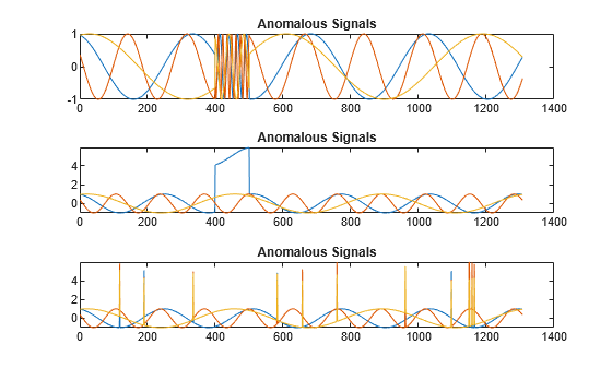
sineWaveAbnormal contains three signals, all of the same length. Each signal in the set has one or more anomalies.

  • All channels of the first signal have an abrupt change in frequency that lasts for a finite time.

  • The second signal has a finite-duration amplitude change in one of its channels.

  • The third signal has spikes at random times in all channels.

Create detector

Use the timeSeriesSpcAD command to create a detector with 3 channels that tracks the exponentially weighted mean average of the data.

detector_tsspc = timeSeriesSpcAD(3, Method="ewma",WindowLength=10);

Train detector

Train the detector using normal data and default settings.

detector_tsspc = train(detector_tsspc,sineWaveNormal)
detector_tsspc = 
  TimeSeriesSPCDetector with properties:

       NumChannels: 3
      WindowLength: 10
            Stride: 10
            Method: "ewma"
            Lambda: 0.4000
    DetectionRules: "n1"
             Level: 3
        CenterLine: [0.0056 -0.0030 -2.9131e-04]
     StandardError: [0.3533 0.3504 0.3538]
              Mean: [0.0056 -0.0030 -2.9131e-04]
             Sigma: [0.7067 0.7008 0.7075]
         MeanRange: [0.1533 0.3004 0.0925]
         IsTrained: 1

Plot detection results

Plot the detection results for sineWaveAbnormal(2)

figure(1);
detector_tsspc.plot(sineWaveAbnormal{2})

Figure contains 3 axes objects. Axes object 1 with title Anomalies, xlabel Samples, ylabel Signal contains 7 objects of type patch, line. These objects represent Labeled Anomalies, Raw Signal (Channel 3), Raw Signal (Channel 2), Raw Signal (Channel 1), Detected Anomalies (Channel 3), Detected Anomalies (Channel 2), Detected Anomalies (Channel 1). Axes object 2 with title EWMA Control Chart, xlabel Window Start Index, ylabel Batch-Means Signal contains 5 objects of type line, constantline. One or more of the lines displays its values using only markers These objects represent Batch-Means Signal (Channel 3), Batch-Means Signal (Channel 2), Batch-Means Signal (Channel 1), Detected Anomalies (across all channels), UCL, CL, LCL. Axes object 3 with title Anomaly Scores, xlabel Window Start Index, ylabel Score contains 3 objects of type stem, line, constantline. One or more of the lines displays its values using only markers These objects represent Anomaly Scores, Detected Anomalies.

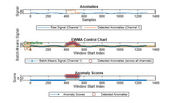
The plot shows that the detector successfully detects the anomaly.

Plot histogram

Plot the histogram of the anomaly scores.

figure(2);
detector_tsspc.plotHistogram(sineWaveNormal{2}, sineWaveAbnormal{2})
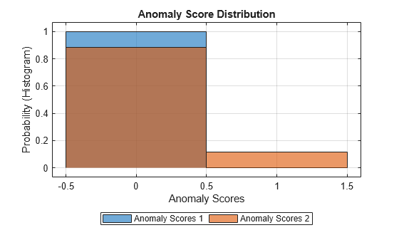
Figure contains an axes object. The axes object with title Anomaly Score Distribution, xlabel Anomaly Scores, ylabel Probability (Histogram) contains 3 objects of type histogram, constantline. These objects represent Anomaly Scores 1, Anomaly Scores 2.

Input Arguments

collapse all

Number of data channels in the input time series for training and detection, specified as a positive integer.

Name-Value Arguments

collapse all

Specify optional pairs of arguments as Name1=Value1,...,NameN=ValueN, where Name is the argument name and Value is the corresponding value. Name-value arguments must appear after other arguments, but the order of the pairs does not matter.

Example: detector = timeSeriesSpcAD(WindowLength=20) sets the length of the detection window to 20.

Length of training and detection window for batch-means computation, specified as a positive integer.

For each window, the detector computes the mean of the data. This reduces autocorrelation of high-frequency data and generates a "shorter" internal time series from which to generate the statistics, such as mean and standard error, that the software applies the control rules to.

Method for detecting anomalies using batch-means data, specified as "individual" or "ewma".

  • When you specify "individual", the detector uses the batch-means data (a time series containing the means of the data windows) to compute and display the control chart statistics.

  • When you specify "ewma", the detector uses the exponentially-weighted batch-means data to compute the control chart parameters and statistics.

Forgetting factor of the EWMA model. The value of Lambda influences the computation results for the standard error.

Number of standard errors around the center line, or mean, of the batch-means data that the software uses to compute default anomalies when the data falls out of this range.

Detection rules, specified as a string vector. Values containing "we" are Western Electric rules, and values containing "n" are Nelson rules. The default rule, which is centerline +/- level*StandardError, is always computed. If you do not want to use the default value, set Level to be a large number.

ValueViolation Condition
"n"All Nelson rules
"we"All Western Electric rules
"n1"

One point below cl 3*se or above cl + 3*se

"n2"Nine of nine points on the same side of cl
"n3"Six of six points increasing or decreasing
"n4"Fourteen points alternating up or down
"n5"

Two of three points below cl 2*se or above cl + 2*se, all on the same side

"n6"

Four of five points below cl se or above cl + se, all on the same side

"n7"

Fifteen of fifteen points between cl se and cl + se

"n8"

Eight of eight points below cl se or above cl + se, on either side

"we1"

One point above cl + 3*se

  
"we3"

Four of five points above cl + se

"we4"Eight of eight points above cl
"we5"

One point below cl 3*se

"we6"

Two of three points below cl 2*se

"we7"

Four of five points below cl se

"we8"Eight of eight points below cl
"we9"

Fifteen of fifteen points between cl se and cl + se

"we10"

Eight of eight points below cl se or above cl + se

For the control rules that involve more than a single point:

  • A rule violation at point i indicates that the set of consecutive points ending at point i triggers the rule. R(i) is true only if point i is one of the points that violates the rule's condition.

  • Any point whose points, center lines, or standard error value is NaN is not counted and always has an R value of false (logical 0).

For more information, see controlrules

Output Arguments

collapse all

Anomaly detector model, returned as an TimeSeriesSPCDetector object.

References

[1] Nelson, Lloyd S. “The Shewhart Control Chart—Tests for Special Causes.” Journal of Quality Technology 16, no. 4 (1984): 237–39. https://doi.org/10.1080/00224065.1984.11978921.

[2] Alexopoulos, Christos, and Andrew F. Seila. “Implementing the Batch Means Method in Simulation Experiments.” Proceedings of the 28th Conference on Winter Simulation - WSC ’96, ACM Press, 1996, 214–21. https://doi.org/10.1145/256562.256608.

[3] Runger, George C., and Thomas R. Willemain. “Batch-Means Control Charts for Autocorrelated Data.” IIE Transactions 28, no. 6 (1996): 483–87. https://doi.org/10.1080/07408179608966295.

[4] Hunter, J. Stuart. “The Exponentially Weighted Moving Average.” Journal of Quality Technology 18, no. 4 (1986): 203–10. https://doi.org/10.1080/00224065.1986.11979014.

Version History

Introduced in R2026a