forecast
Forecast univariate ARIMA or ARIMAX model responses or conditional variances
Syntax
Description
[
returns the Y,YMSE]
= forecast(Mdl,numperiods,Y0)numperiods-by-1 numeric vector of consecutive forecasted
responses Y and the corresponding numeric vector of forecast mean
square errors (MSE) YMSE of the fully specified, univariate ARIMA model
Mdl. The presample response data in the numeric vector
Y0 initializes the model to generate forecasts.
Tbl2 = forecast(Mdl,numperiods,Tbl1)Tbl2 containing a variable for each of
the paths of response, forecast MSE, and conditional variance series resulting from
forecasting the ARIMA model Mdl over a numperiods
forecast horizon. Tbl1 is a table or timetable containing a variable
for required presample response data to initialize the model for forecasting.
Tbl1 can optionally contain variables of presample data for
innovations, conditional variances, and predictors. (since R2023b)
forecast selects the response variable named in
Mdl.SeriesName or the sole variable in Tbl1. To
select a different response variable in Tbl1 to initialize the model,
use the PresampleResponseVariable name-value argument.
[___] = forecast(___,
specifies options using one or more name-value arguments in
addition to any of the input argument combinations in previous syntaxes.
Name=Value)forecast returns the output argument combination for the
corresponding input arguments. For example, forecast(Mdl,10,Y0,X0=Exo0,XF=Exo) specifies
the presample and forecast sample exogenous predictor data to Exo0 and
Exo, respectively, to forecast a model with a regression component
(an ARIMAX model).
Examples
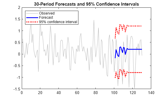
Forecast the conditional mean response of simulated data over a 30-period horizon. Supply a vector of presample response data and return a vector of forecasts.
Simulate 130 observations from a multiplicative seasonal moving average (MA) model with known parameter values.
Mdl = arima(MA={0.5 -0.3},SMA=0.4,SMALags=12,Constant=0.04, ...
    Variance=0.2);
rng(200,"twister")
Y = simulate(Mdl,130);
Fit a seasonal MA model to the first 100 observations, and reserve the remaining 30 observations to evaluate forecast performance.
MdlTemplate = arima(MALags=1:2,SMALags=12);
EstMdl = estimate(MdlTemplate,Y(1:100));
    ARIMA(0,0,2) Model with Seasonal MA(12) (Gaussian Distribution):

                 Value      StandardError    TStatistic      PValue
                ________    _____________    __________    __________

    Constant     0.20403      0.069064         2.9542       0.0031344
    MA{1}        0.50212      0.097298         5.1606      2.4619e-07
    MA{2}       -0.20174       0.10447        -1.9312        0.053464
    SMA{12}      0.27028       0.10907          2.478        0.013211
    Variance     0.18681      0.032732         5.7073       1.148e-08
EstMdl is a new arima model that contains estimated parameters (that is, a fully specified model).
Forecast the fitted model into a 30-period horizon. Specify the estimation period data as a presample.
[YF,YMSE] = forecast(EstMdl,30,Y(1:100));

YF(15)
ans =
0.2040
YMSE(15)
ans =
0.2592
YF is a 30-by-1 vector of forecasted responses, and YMSE is a 30-by-1 vector of corresponding MSEs. The 15-period-ahead forecast is 0.2040 and its MSE is 0.2592.
Visually compare the forecasts to the holdout data.
figure
h1 = plot(Y,Color=[.7,.7,.7]);
hold on
h2 = plot(101:130,YF,"b",LineWidth=2);
h3 = plot(101:130,YF + 1.96*sqrt(YMSE),"r:",LineWidth=2);
plot(101:130,YF - 1.96*sqrt(YMSE),"r:",LineWidth=2);
legend([h1 h2 h3],"Observed","Forecast","95% confidence interval", ...
    Location="NorthWest")
title("30-Period Forecasts and 95% Confidence Intervals")
hold off
Since R2023b
Forecast the weekly average NYSE closing prices over a 15-week horizon. Supply presample data in a timetable and return a timetable of forecasts.
Load Data
Load the US equity index data set Data_EquityIdx.
load Data_EquityIdx
T = height(DataTimeTable)
T = 3028
The timetable DataTimeTable includes the time series variable NYSE, which contains daily NYSE composite closing prices from January 1990 through December 2001.
Plot the daily NYSE price series.
figure
plot(DataTimeTable.Time,DataTimeTable.NYSE)
title("NYSE Daily Closing Prices: 1990 - 2001")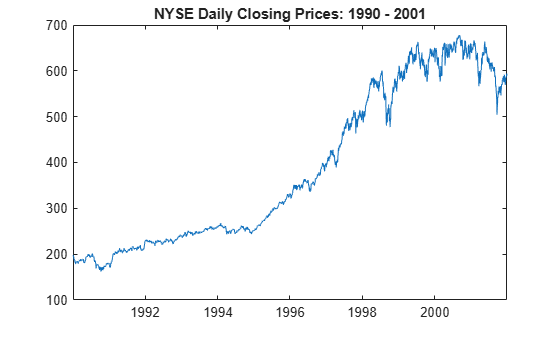
Prepare Timetable for Estimation
When you plan to supply a timetable, you must ensure it has all the following characteristics:
The selected response variable is numeric and does not contain any missing values.
The timestamps in the
Timevariable are regular, and they are ascending or descending.
Remove all missing values from the timetable, relative to the NYSE price series.
DTT = rmmissing(DataTimeTable,DataVariables="NYSE");
T_DTT = height(DTT)
T_DTT = 3028
Because all sample times have observed NYSE prices, rmmissing does not remove any observations.
Determine whether the sampling timestamps have a regular frequency and are sorted.
areTimestampsRegular = isregular(DTT,"days")areTimestampsRegular = logical
0
areTimestampsSorted = issorted(DTT.Time)
areTimestampsSorted = logical
   1
areTimestampsRegular = 0 indicates that the timestamps of DTT are irregular. areTimestampsSorted = 1 indicates that the timestamps are sorted. Business day rules make daily macroeconomic measurements irregular.
Remedy the time irregularity by computing the weekly average closing price series of all timetable variables.
DTTW = convert2weekly(DTT,Aggregation="mean");
areTimestampsRegular = isregular(DTTW,"weeks")
areTimestampsRegular = logical
   1
T_DTTW = height(DTTW)
T_DTTW =
627
DTTW is regular.
figure
plot(DTTW.Time,DTTW.NYSE)
title("NYSE Daily Closing Prices: 1990 - 2001")
Create Model Template for Estimation
Suppose that an ARIMA(1,1,1) model is appropriate to model NYSE composite series during the sample period.
Create an ARIMA(1,1,1) model template for estimation. Set the response series name to NYSE.
Mdl = arima(1,1,1);
Mdl.SeriesName = "NYSE";
Mdl is a partially specified arima model object.
Partition Data
estimate and forecast require Mdl.P presample observations to initialize the model for estimation and forecasting.
Partition the data into three sets:
A presample set for estimation
An in-sample set, to which you fit the model and initialize the model for forecasting
A holdout sample of length 15 to measure the model's predictive performance
numpreobs = Mdl.P;                  % Required presample length
numperiods = 15;                    % Forecast horizon
DTTW0 = DTTW(1:numpreobs,:);        % Estimation presample
DTTW1 = DTTW((numpreobs+1):(end-numperiods),:);
    % In-sample for estimation and presample for forecasting
    DTTW2 = DTTW((end-numperiods+1):end,:); % Holdout sample
Fit Model to Data
Fit an ARIMA(1,1,1) model to the in-sample weekly average NYSE closing prices. Specify the presample timetable and the presample response variable name.
EstMdl = estimate(Mdl,DTTW1,Presample=DTTW0,PresampleResponseVariable="NYSE");
    ARIMA(1,1,1) Model (Gaussian Distribution):

                 Value      StandardError    TStatistic      PValue
                ________    _____________    __________    ___________

    Constant     0.31873       0.23754         1.3418          0.17965
    AR{1}        0.41132        0.2371         1.7348         0.082781
    MA{1}       -0.31232       0.24486        -1.2755          0.20213
    Variance      55.472        1.8496         29.992      1.2639e-197
EstMdl is a fully specified, estimated arima model object.
Forecast Conditional Mean
Forecast the weekly average NASDQ closing prices 15 weeks beyond the estimation sample using the fitted model. Use the estimation sample data as a presample to initialize the forecast. Specify the response variable name in the presample data.
Tbl2 = forecast(EstMdl,numperiods,DTTW1)
Tbl2=15×3 timetable
       Time        NYSE_Response    NYSE_MSE    NYSE_Variance
    ___________    _____________    ________    _____________

    28-Sep-2001       521.34         55.472        55.472
    05-Oct-2001       519.89         122.47        55.472
    12-Oct-2001       519.62         194.53        55.472
    19-Oct-2001       519.82         268.72        55.472
    26-Oct-2001       520.23          343.8        55.472
    02-Nov-2001       520.71         419.24        55.472
    09-Nov-2001       521.23         494.83        55.472
    16-Nov-2001       521.76         570.49        55.472
    23-Nov-2001        522.3         646.17        55.472
    30-Nov-2001       522.84         721.86        55.472
    07-Dec-2001       523.38         797.56        55.472
    14-Dec-2001       523.92         873.26        55.472
    21-Dec-2001       524.46         948.96        55.472
    28-Dec-2001          525         1024.7        55.472
    04-Jan-2002       525.55         1100.4        55.472
Tbl2 is a 15-by-3 timetable containing the forecasted weekly average closing price forecasts NYSE_Response, corresponding forecast MSEs NYSE_MSE, and the model's constant variance NYSE_Variance (EstMdl.Variance = 55.8147).
Plot the forecasts and approximate 95% forecast intervals.
Tbl2.NYSE_Lower = Tbl2.NYSE_Response - 1.96*sqrt(Tbl2.NYSE_MSE);
Tbl2.NYSE_Upper = Tbl2.NYSE_Response + 1.96*sqrt(Tbl2.NYSE_MSE);

figure
h1 = plot([DTTW1.Time((end-75):end); DTTW2.Time], ...
    [DTTW1.NYSE((end-75):end); DTTW2.NYSE],Color=[.7,.7,.7]);
hold on
h2 = plot(Tbl2.Time,Tbl2.NYSE_Response,"k",LineWidth=2);
h3 = plot(Tbl2.Time,Tbl2{:,["NYSE_Lower" "NYSE_Upper"]},"r:",LineWidth=2);
legend([h1 h2 h3(1)],"Observations","Forecasts","95% forecast intervals", ...
    Location="NorthWest")
title("NYSE Weekly Average Closing Price")
hold off

The process is nonstationary, so the width of each forecast interval grows with time. The model tends to underestimate the weekly average closing prices.
Forecast the following known autoregressive model with one lag and an exogenous predictor (ARX(1)) model into a 10-period forecast horizon:
where is a standard Gaussian random variable, and is an exogenous Gaussian random variable with a mean of 1 and a standard deviation of 0.5.
Create an arima model object that represents the ARX(1) model.
Mdl = arima(Constant=1,AR=0.3,Beta=2,Variance=1);
To forecast responses from the ARX(1) model, the forecast function requires:
One presample response to initialize the autoregressive term
Future exogenous data to include the effects of the exogenous variable on the forecasted responses
Set the presample response to the unconditional mean of the stationary process:
For the future exogenous data, draw 10 values from the distribution of the exogenous variable.
rng(1,"twister");
y0 = (1 + 2)/(1 - 0.3);
xf = 1 + 0.5*randn(10,1);
Forecast the ARX(1) model into a 10-period forecast horizon. Specify the presample response and future exogenous data.
fh = 10;
yf = forecast(Mdl,fh,y0,XF=xf)
yf = 10×1

    3.6367
    5.2722
    3.8232
    3.0373
    3.0657
    3.3470
    3.4454
    4.2120
    4.0667
    4.8065
yf(3) = 3.8232 is the 3-period-ahead forecast of the ARX(1) model.
Since R2023b
Consider the following AR(1) conditional mean model with a GARCH(1,1) conditional variance model for the weekly average NASDAQ rate series (as a percent) from January 2, 1990 through December 31, 2001.
where is a series of independent random Gaussian variables with a mean of 0.
Create the model. Name the response series NASDAQ.
CondVarMdl = garch(Constant=0.022,GARCH=0.873,ARCH=0.119);
Mdl = arima(Constant=0.073,AR=0.138,Variance=CondVarMdl);
Mdl.SeriesName = "NASDAQ";
Load the equity index data set. Remedy the time irregularity by computing the weekly average closing price series of all timetable variables.
load Data_EquityIdx
DTTW = convert2weekly(DataTimeTable,Aggregation="mean");
Convert the weekly average NASDAQ closing price series to a percent return series.
RetTT = price2ret(DTTW);
RetTT.NASDAQ = RetTT.NASDAQ*100;
Infer residuals and conditional variances from the model.
RetTT2 = infer(Mdl,RetTT);
T = numel(RetTT);
Forecast the model over a 25-day horizon. Supply the entire data set as a presample (forecast uses only the latest required observations to initialize the conditional mean and variance models). Supply variable names for the presample innovations and conditional variances. By default, forecast uses the variable name Mdl.SeriesName as the presample response variable.
fh = 25;
ForecastTT = forecast(Mdl,fh,RetTT2,PresampleInnovationVariable="NASDAQ_Residual", ...
    PresampleVarianceVariable="NASDAQ_Variance");
Plot the forecasted responses and conditional variances with the observed series from June 2000.
pdates = RetTT2.Time > datetime(2000,6,1);

figure
plot(RetTT2.Time(pdates),RetTT2.NASDAQ(pdates))
hold on
plot([RetTT2.Time(end); ForecastTT.Time], ...
    [RetTT2.NASDAQ(end); ForecastTT.NASDAQ_Response])
title("NASDAQ Weekly Average Percent Return Series")
legend("Observed","Forecasted")
axis tight
grid on
hold off
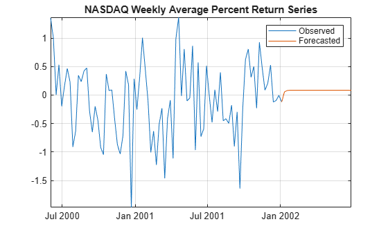
figure
plot(RetTT2.Time(pdates),RetTT2.NASDAQ_Variance(pdates))
hold on
plot([RetTT2.Time(end); ForecastTT.Time], ...
    [RetTT2.NASDAQ_Variance(end); ForecastTT.NASDAQ_Variance])
title("Conditional Variance Series")
legend("Observed","Forecasted")
axis tight
grid on
hold off

Forecast multiple response and conditional variance paths from a known composite conditional mean and variance model: a SAR conditional mean model with an ARCH(1) conditional variance model. Specify multiple presample response paths.
Create a garch model object that represents this ARCH(1) model:
Create an arima model object that represents this quarterly SAR model:
where is a standard Gaussian random variable.
CVMdl = garch(ARCH=0.2,Constant=0.1)
CVMdl =
  garch with properties:

     Description: "GARCH(0,1) Conditional Variance Model (Gaussian Distribution)"
      SeriesName: "Y"
    Distribution: Name = "Gaussian"
               P: 0
               Q: 1
        Constant: 0.1
           GARCH: {}
            ARCH: {0.2} at lag [1]
          Offset: 0
Mdl = arima(Constant=1,AR=0.5,Variance=CVMdl,Seasonality=4, ...
    SARLags=4,SAR=0.2)
Mdl =
arima with properties:
Description: "ARIMA(1,0,0) Model Seasonally Integrated with Seasonal AR(4) (Gaussian Distribution)"
SeriesName: "Y"
Distribution: Name = "Gaussian"
P: 9
D: 0
Q: 0
Constant: 1
AR: {0.5} at lag [1]
SAR: {0.2} at lag [4]
MA: {}
SMA: {}
Seasonality: 4
Beta: [1×0]
Variance: [GARCH(0,1) Model]
Because Mdl contains 9 autoregressive terms and 1 ARCH term, forecast requires Mdl.P = 9 responses and CVMdl.Q = 1 conditional variance to generate each -period-ahead forecast.
Generate 10 random paths of length 9 from the model.
rng(1,"twister")
numpreobs = Mdl.P;
numpaths = 10;
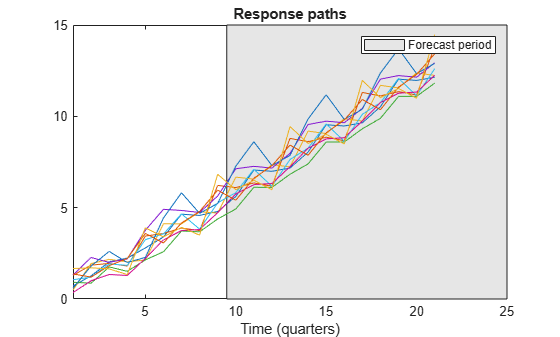
[Y0,~,V0] = simulate(Mdl,numpreobs,NumPaths=numpaths);Forecast 10 paths of responses and conditional variances from the model into a 12-quarter forecast horizon. Specify the presample response paths Y0 and conditional variance paths V0.
fh = 12;
[YF,~,VF] = forecast(Mdl,fh,Y0,V0=V0);
YF and VF are 12-by-10 matrices of independent forecasted response and conditional variance paths, respectively. YF(j,k) is the j-period-ahead forecast of path k. Path YF(:,k) represents the continuation of the presample path Y0(:,k). forecast structures VF similarly.
Plot the presample and forecasted responses.
Y = [Y0; YF];

figure
plot(Y)
hold on
h = gca;
px = [numpreobs+0.5 h.XLim([2 2]) numpreobs+0.5];
py = h.YLim([1 1 2 2]);
hp = patch(px,py,[0.9 0.9 0.9]);
uistack(hp,"bottom");
axis tight
legend("Forecast period")
xlabel("Time (quarters)")
title("Response paths")
hold off
V = [V0; VF];

figure
plot(V)
hold on
h = gca;
px = [numpreobs+0.5 h.XLim([2 2]) numpreobs+0.5];
py = h.YLim([1 1 2 2]);
hp = patch(px,py,[0.9 0.9 0.9]);
uistack(hp,"bottom");
legend("Forecast period")
axis tight
xlabel("Time (quarters)")
title("Conditional Variance Paths")
hold off

Input Arguments
Name-Value Arguments
Output Arguments
More About
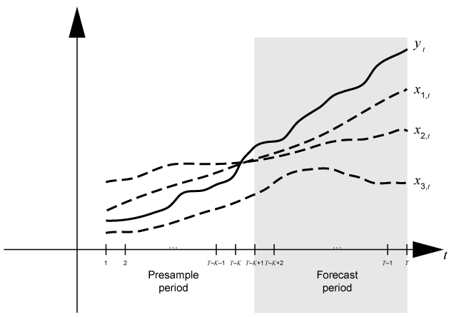
Time base partitions for forecasting are two
disjoint, contiguous intervals of the time base; each interval contains time series data for
forecasting a dynamic model. The forecast period (forecast horizon)
is a numperiods length partition at the end of the time base during
which the forecast function generates the forecasts
Y from the dynamic model Mdl. The
presample period is the entire partition occurring before the
forecast period. The forecast function can require observed
responses, innovations, or conditional variances in the presample period
(Y0, E0, and V0, or
Tbl1) to initialize the dynamic model for forecasting. The model
structure determines the types and amounts of required presample observations.
A common practice is to fit a dynamic model to a portion of the data set, and then validate the predictability of the model by comparing its forecasts to observed responses. During forecasting, the presample period contains the data to which the model is fit, and the forecast period contains the holdout sample for validation. Suppose that yt is an observed response series; x1,t, x2,t, and x3,t are observed exogenous series; and time t = 1,…,T. Consider forecasting responses from a dynamic model of yt containing a regression component with numperiods = K periods. Suppose that the dynamic model is fit to the data in the interval [1,T – K] (for more details, see estimate). This figure shows the time base partitions for forecasting.
For example, to generate the forecasts Y from an ARX(2) model, forecast requires:
Presample responses
Y0= to initialize the model. The 1-period-ahead forecast requires both observations, whereas the 2-periods-ahead forecast requires yT – K and the 1-period-ahead forecastY(1). Theforecastfunction generates all other forecasts by substituting previous forecasts for lagged responses in the model.Future exogenous data
XF= for the model regression component. Without specified future exogenous data, theforecastfunction ignores the model regression component, which can yield unrealistic forecasts.
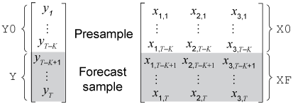
Dynamic models containing either a moving average component or a conditional variance model can require presample innovations or conditional variances. Given enough presample responses, forecast infers the required presample innovations and conditional variances. If such a model also contains a regression component, then forecast must have enough presample responses and exogenous data to infer the required presample innovations and conditional variances. This figure shows the arrays of required observations for this case, with corresponding input and output arguments.
Algorithms
The
forecastfunction sets the number of sample paths (numpaths) to the maximum number of columns among the specified presample data sets:For input numeric arrays of presample data,
numpathsis the maximum width amongE0,V0, andY0.For an input table or timetable of presample data,
numpathsis the maximum width among the variables representing the presample responsesPresampleResponseVariable, innovationsPresampleInnovationVariable, and conditional variancesPresampleVarianceVariable.
All specified presample data sets must have either one column or
numpaths> 1 columns. Otherwise,forecastissues an error. For example, if you supplyY0andE0, andY0has five columns representing five paths, thenE0can have one column or five columns. IfE0has one column,forecastappliesE0to each path.NaNvalues in presample and future data sets indicate missing data. For input numeric arrays,forecastremoves missing data from the presample data sets following this procedure:forecasthorizontally concatenates the specified presample data setsY0,E0,V0, andX0so that the latest observations occur simultaneously. The result can be a jagged array because the presample data sets can have a different number of rows. In this case,forecastprepads variables with an appropriate number of zeros to form a matrix.forecastapplies listwise deletion to the combined presample matrix by removing all rows containing at least oneNaN.forecastextracts the processed presample data sets from the result of step 2, and removes all prepadded zeros.
forecastapplies a similar procedure to the forecasted predictor dataXF. Afterforecastapplies listwise deletion toXF, the result must have at leastnumperiodsrows. Otherwise,forecastissues an error.List-wise deletion reduces the sample size and can create irregular time series.
forecastissues an error when any table or timetable input contains missing values.When
forecastcomputes the MSEsYMSEof the conditional mean forecastsY, the function treats the specified predictor data sets as exogenous, nonstochastic, and statistically independent of the model innovations. Therefore,YMSEreflects only the variance associated with the ARIMA component of the input modelMdl.
References
[1] Baillie, Richard T., and Tim Bollerslev. “Prediction in Dynamic Models with Time-Dependent Conditional Variances.” Journal of Econometrics 52, (April 1992): 91–113. https://doi.org/10.1016/0304-4076(92)90066-Z.
[2] Bollerslev, Tim. “Generalized Autoregressive Conditional Heteroskedasticity.” Journal of Econometrics 31 (April 1986): 307–27. https://doi.org/10.1016/0304-4076(86)90063-1.
[3] Bollerslev, Tim. “A Conditionally Heteroskedastic Time Series Model for Speculative Prices and Rates of Return.” The Review of Economics and Statistics 69 (August 1987): 542–47. https://doi.org/10.2307/1925546.
[4] Box, George E. P., Gwilym M. Jenkins, and Gregory C. Reinsel. Time Series Analysis: Forecasting and Control. 3rd ed. Englewood Cliffs, NJ: Prentice Hall, 1994.
[5] Enders, Walter. Applied Econometric Time Series. Hoboken, NJ: John Wiley & Sons, Inc., 1995.
[6] Engle, Robert. F. “Autoregressive Conditional Heteroscedasticity with Estimates of the Variance of United Kingdom Inflation.” Econometrica 50 (July 1982): 987–1007. https://doi.org/10.2307/1912773.
[7] Hamilton, James D. Time Series Analysis. Princeton, NJ: Princeton University Press, 1994.