yamnet

(非推奨) YAMNet ニューラル ネットワーク

yamnet は推奨されません。代わりに audioPretrainedNetwork (Audio Toolbox) 関数を使用してください。

構文

net = yamnet

説明

net = yamnet は、事前学習済みの YAMNet モデルを返します。

この関数には、Audio Toolbox™ と Deep Learning Toolbox™ の両方が必要です。

例

YAMNet のダウンロード

YAMNet 用の Audio Toolbox™ モデルをダウンロードして解凍します。

コマンド ウィンドウで yamnet と入力します。YAMNet 用の Audio Toolbox モデルがインストールされていない場合、この関数はネットワークの重みファイルの場所へのリンクを提供します。モデルをダウンロードするには、リンクをクリックします。MATLAB パス上の場所にファイルを解凍します。

または、次のコマンドを実行し、YAMNet モデルを一時ディレクトリにダウンロードして解凍します。

downloadFolder = fullfile(tempdir,'YAMNetDownload');
loc = websave(downloadFolder,'https://ssd.mathworks.com/supportfiles/audio/yamnet.zip');
YAMNetLocation = tempdir;
unzip(loc,YAMNetLocation)
addpath(fullfile(YAMNetLocation,'yamnet'))

コマンド ウィンドウで yamnet と入力して、インストールが正常に終了していることを確認します。ネットワークがインストールされている場合、関数はSeriesNetworkオブジェクトを返します。

yamnet

ans = 
  SeriesNetwork with properties:

         Layers: [86×1 nnet.cnn.layer.Layer]
     InputNames: {'input_1'}
    OutputNames: {'Sound'}

事前学習済みの YAMNet の読み込み

事前学習済みの YAMNet 畳み込みニューラル ネットワークを読み込み、層とクラスを調べます。

yamnet を使用して、事前学習済みの YAMNet ネットワークを読み込みます。出力される net はSeriesNetworkオブジェクトです。

net = yamnet

net = 
  SeriesNetwork with properties:

         Layers: [86×1 nnet.cnn.layer.Layer]
     InputNames: {'input_1'}
    OutputNames: {'Sound'}

Layers プロパティを使用してネットワーク アーキテクチャを表示します。このネットワークには 86 個の層があります。学習可能な重みをもつ層が 28 個あります。27 個は畳み込み層で、1 個は全結合層です。

net.Layers

ans = 
  86x1 Layer array with layers:

     1   'input_1'                    Image Input              96×64×1 images
     2   'conv2d'                     Convolution              32 3×3×1 convolutions with stride [2  2] and padding 'same'
     3   'b'                          Batch Normalization      Batch normalization with 32 channels
     4   'activation'                 ReLU                     ReLU
     5   'depthwise_conv2d'           Grouped Convolution      32 groups of 1 3×3×1 convolutions with stride [1  1] and padding 'same'
     6   'L11'                        Batch Normalization      Batch normalization with 32 channels
     7   'activation_1'               ReLU                     ReLU
     8   'conv2d_1'                   Convolution              64 1×1×32 convolutions with stride [1  1] and padding 'same'
     9   'L12'                        Batch Normalization      Batch normalization with 64 channels
    10   'activation_2'               ReLU                     ReLU
    11   'depthwise_conv2d_1'         Grouped Convolution      64 groups of 1 3×3×1 convolutions with stride [2  2] and padding 'same'
    12   'L21'                        Batch Normalization      Batch normalization with 64 channels
    13   'activation_3'               ReLU                     ReLU
    14   'conv2d_2'                   Convolution              128 1×1×64 convolutions with stride [1  1] and padding 'same'
    15   'L22'                        Batch Normalization      Batch normalization with 128 channels
    16   'activation_4'               ReLU                     ReLU
    17   'depthwise_conv2d_2'         Grouped Convolution      128 groups of 1 3×3×1 convolutions with stride [1  1] and padding 'same'
    18   'L31'                        Batch Normalization      Batch normalization with 128 channels
    19   'activation_5'               ReLU                     ReLU
    20   'conv2d_3'                   Convolution              128 1×1×128 convolutions with stride [1  1] and padding 'same'
    21   'L32'                        Batch Normalization      Batch normalization with 128 channels
    22   'activation_6'               ReLU                     ReLU
    23   'depthwise_conv2d_3'         Grouped Convolution      128 groups of 1 3×3×1 convolutions with stride [2  2] and padding 'same'
    24   'L41'                        Batch Normalization      Batch normalization with 128 channels
    25   'activation_7'               ReLU                     ReLU
    26   'conv2d_4'                   Convolution              256 1×1×128 convolutions with stride [1  1] and padding 'same'
    27   'L42'                        Batch Normalization      Batch normalization with 256 channels
    28   'activation_8'               ReLU                     ReLU
    29   'depthwise_conv2d_4'         Grouped Convolution      256 groups of 1 3×3×1 convolutions with stride [1  1] and padding 'same'
    30   'L51'                        Batch Normalization      Batch normalization with 256 channels
    31   'activation_9'               ReLU                     ReLU
    32   'conv2d_5'                   Convolution              256 1×1×256 convolutions with stride [1  1] and padding 'same'
    33   'L52'                        Batch Normalization      Batch normalization with 256 channels
    34   'activation_10'              ReLU                     ReLU
    35   'depthwise_conv2d_5'         Grouped Convolution      256 groups of 1 3×3×1 convolutions with stride [2  2] and padding 'same'
    36   'L61'                        Batch Normalization      Batch normalization with 256 channels
    37   'activation_11'              ReLU                     ReLU
    38   'conv2d_6'                   Convolution              512 1×1×256 convolutions with stride [1  1] and padding 'same'
    39   'L62'                        Batch Normalization      Batch normalization with 512 channels
    40   'activation_12'              ReLU                     ReLU
    41   'depthwise_conv2d_6'         Grouped Convolution      512 groups of 1 3×3×1 convolutions with stride [1  1] and padding 'same'
    42   'L71'                        Batch Normalization      Batch normalization with 512 channels
    43   'activation_13'              ReLU                     ReLU
    44   'conv2d_7'                   Convolution              512 1×1×512 convolutions with stride [1  1] and padding 'same'
    45   'L72'                        Batch Normalization      Batch normalization with 512 channels
    46   'activation_14'              ReLU                     ReLU
    47   'depthwise_conv2d_7'         Grouped Convolution      512 groups of 1 3×3×1 convolutions with stride [1  1] and padding 'same'
    48   'L81'                        Batch Normalization      Batch normalization with 512 channels
    49   'activation_15'              ReLU                     ReLU
    50   'conv2d_8'                   Convolution              512 1×1×512 convolutions with stride [1  1] and padding 'same'
    51   'L82'                        Batch Normalization      Batch normalization with 512 channels
    52   'activation_16'              ReLU                     ReLU
    53   'depthwise_conv2d_8'         Grouped Convolution      512 groups of 1 3×3×1 convolutions with stride [1  1] and padding 'same'
    54   'L91'                        Batch Normalization      Batch normalization with 512 channels
    55   'activation_17'              ReLU                     ReLU
    56   'conv2d_9'                   Convolution              512 1×1×512 convolutions with stride [1  1] and padding 'same'
    57   'L92'                        Batch Normalization      Batch normalization with 512 channels
    58   'activation_18'              ReLU                     ReLU
    59   'depthwise_conv2d_9'         Grouped Convolution      512 groups of 1 3×3×1 convolutions with stride [1  1] and padding 'same'
    60   'L101'                       Batch Normalization      Batch normalization with 512 channels
    61   'activation_19'              ReLU                     ReLU
    62   'conv2d_10'                  Convolution              512 1×1×512 convolutions with stride [1  1] and padding 'same'
    63   'L102'                       Batch Normalization      Batch normalization with 512 channels
    64   'activation_20'              ReLU                     ReLU
    65   'depthwise_conv2d_10'        Grouped Convolution      512 groups of 1 3×3×1 convolutions with stride [1  1] and padding 'same'
    66   'L111'                       Batch Normalization      Batch normalization with 512 channels
    67   'activation_21'              ReLU                     ReLU
    68   'conv2d_11'                  Convolution              512 1×1×512 convolutions with stride [1  1] and padding 'same'
    69   'L112'                       Batch Normalization      Batch normalization with 512 channels
    70   'activation_22'              ReLU                     ReLU
    71   'depthwise_conv2d_11'        Grouped Convolution      512 groups of 1 3×3×1 convolutions with stride [2  2] and padding 'same'
    72   'L121'                       Batch Normalization      Batch normalization with 512 channels
    73   'activation_23'              ReLU                     ReLU
    74   'conv2d_12'                  Convolution              1024 1×1×512 convolutions with stride [1  1] and padding 'same'
    75   'L122'                       Batch Normalization      Batch normalization with 1024 channels
    76   'activation_24'              ReLU                     ReLU
    77   'depthwise_conv2d_12'        Grouped Convolution      1024 groups of 1 3×3×1 convolutions with stride [1  1] and padding 'same'
    78   'L131'                       Batch Normalization      Batch normalization with 1024 channels
    79   'activation_25'              ReLU                     ReLU
    80   'conv2d_13'                  Convolution              1024 1×1×1024 convolutions with stride [1  1] and padding 'same'
    81   'L132'                       Batch Normalization      Batch normalization with 1024 channels
    82   'activation_26'              ReLU                     ReLU
    83   'global_average_pooling2d'   Global Average Pooling   Global average pooling
    84   'dense'                      Fully Connected          521 fully connected layer
    85   'softmax'                    Softmax                  softmax
    86   'Sound'                      Classification Output    crossentropyex with 'Speech' and 520 other classes

ネットワークが学習したクラスの名前を表示するには、分類出力層 (最後の層) の Classes プロパティを表示します。最初の 10 個の要素を指定し、最初の 10 個のクラスを表示します。

net.Layers(end).Classes(1:10)

ans = 10×1 categorical
     Speech 
     Child speech, kid speaking 
     Conversation 
     Narration, monologue 
     Babbling 
     Speech synthesizer 
     Shout 
     Bellow 
     Whoop 
     Yell 

analyzeNetworkを使用して、ネットワークを視覚的に確認します。

analyzeNetwork(net)

YAMNet は、対応するサウンド クラスのオントロジーと共にリリースされており、yamnetGraph (Audio Toolbox)オブジェクトを使用して確認できます。

ygraph = yamnetGraph;
p = plot(ygraph);
layout(p,'layered')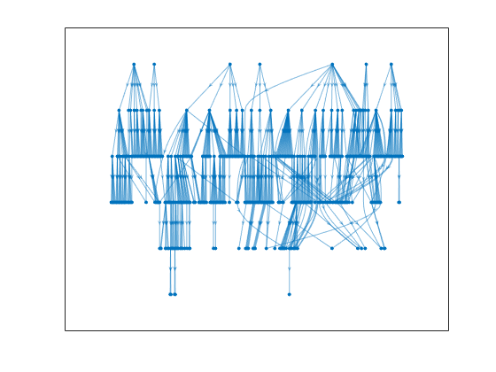

オントロジーのグラフには、考えられる 521 個のサウンド クラスがすべてプロットされます。呼吸音に関する音の部分グラフをプロットします。

allRespiratorySounds = dfsearch(ygraph,"Respiratory sounds");
ygraphSpeech = subgraph(ygraph,allRespiratorySounds);
plot(ygraphSpeech)

YAMNet を使用した音の分類

オーディオ信号を読み取って分類します。

[audioIn,fs] = audioread("TrainWhistle-16-44p1-mono-9secs.wav");

オーディオ信号をプロットして再生します。

t = (0:numel(audioIn)-1)/fs;
plot(t,audioIn)
xlabel("Time (s)")
ylabel("Ampltiude")
axis tight

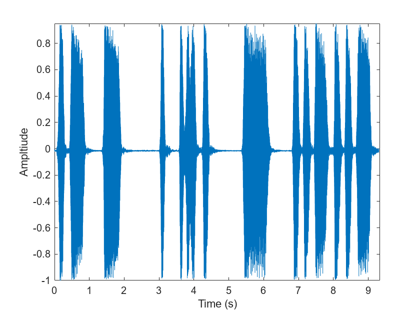
sound(audioIn,fs)

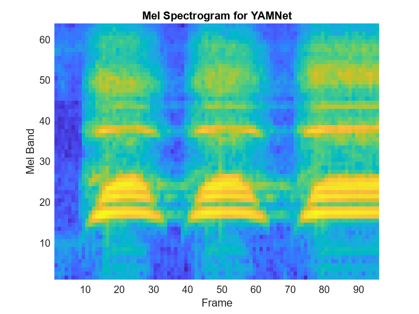
YAMNet では、ネットワークの学習に使用される入力形式に合わせてオーディオ信号を前処理する必要があります。この前処理手順では、オーディオ信号のリサンプリングとメル スペクトログラムの配列の計算を行います。メル スペクトログラムの詳細については、melSpectrogram (Audio Toolbox)を参照してください。yamnetPreprocess を使用して信号を前処理し、YAMNet に渡すメル スペクトログラムを抽出します。これらのスペクトログラムの 1 つをランダムに選択して可視化します。

spectrograms = yamnetPreprocess(audioIn,fs);

arbitrarySpect = spectrograms(:,:,1,randi(size(spectrograms,4)));
surf(arbitrarySpect,EdgeColor="none")
view([90 -90])
xlabel("Mel Band")
ylabel("Frame")
title("Mel Spectrogram for YAMNet")
axis tight

audioPretrainedNetwork 関数を使用して、YAMNet ニューラル ネットワークを作成します。前処理されたメル スペクトログラム イメージに対し、ネットワークで predict を呼び出します。scores2label を使用して、ネットワークの出力をクラス ラベルに変換します。

[net,classNames] = audioPretrainedNetwork("yamnet");
scores = predict(net,spectrograms);
classes = scores2label(scores,classNames);

この分類手順では、入力に含まれる各スペクトログラム イメージのラベルが返されます。出力内で最も頻繁に出現するラベルとしてサウンドを分類します。

mySound = mode(classes)

mySound = categorical
     Whistle 

YAMNet を使用した転移学習

エアー コンプレッサーのデータ セット [1] をダウンロードして解凍します。このデータ セットは、正常な状態または 7 つの故障状態のいずれかにあるコンプレッサーから得られた記録で構成されています。

url = "https://www.mathworks.com/supportfiles/audio/AirCompressorDataset/AirCompressorDataset.zip";
downloadFolder = fullfile(tempdir,"aircompressordataset");
datasetLocation = tempdir;

if ~exist(fullfile(tempdir,"AirCompressorDataSet"),"dir")
    loc = websave(downloadFolder,url);
    unzip(loc,fullfile(tempdir,"AirCompressorDataSet"))
end

データを管理するためのaudioDatastore (Audio Toolbox)オブジェクトを作成し、学習セットと検証セットに分割します。

ads = audioDatastore(downloadFolder,IncludeSubfolders=true,LabelSource="foldernames");

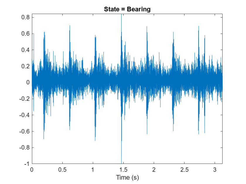
[adsTrain,adsValidation] = splitEachLabel(ads,0.8,0.2);

データストアからオーディオ ファイルを読み取り、後で使用するためにサンプル レートを保存します。データストアをリセットし、読み取りポインターをデータ セットの先頭に戻します。オーディオ信号を再生し、その信号を時間領域でプロットします。

[x,fileInfo] = read(adsTrain);
fs = fileInfo.SampleRate;

reset(adsTrain)

sound(x,fs)

figure
t = (0:size(x,1)-1)/fs;
plot(t,x)
xlabel("Time (s)")
title("State = " + string(fileInfo.Label))
axis tight

yamnetPreprocess を使用して、学習セットからメル スペクトログラムを抽出します。各オーディオ信号に対して複数のスペクトログラムが存在します。スペクトログラムと 1 対 1 で対応するように、ラベルを複製します。

emptyLabelVector = adsTrain.Labels;
emptyLabelVector(:) = [];

trainFeatures = [];
trainLabels = emptyLabelVector;
while hasdata(adsTrain)
    [audioIn,fileInfo] = read(adsTrain);
    features = yamnetPreprocess(audioIn,fileInfo.SampleRate);
    numSpectrums = size(features,4);
    trainFeatures = cat(4,trainFeatures,features);
    trainLabels = cat(2,trainLabels,repmat(fileInfo.Label,1,numSpectrums));
end

検証セットから特徴を抽出し、ラベルを複製します。

validationFeatures = [];
validationLabels = emptyLabelVector;
while hasdata(adsValidation)
    [audioIn,fileInfo] = read(adsValidation);
    features = yamnetPreprocess(audioIn,fileInfo.SampleRate);
    numSpectrums = size(features,4);
    validationFeatures = cat(4,validationFeatures,features);
    validationLabels = cat(2,validationLabels,repmat(fileInfo.Label,1,numSpectrums));
end

コンプレッサー データ セットには 8 つのクラスしかありません。NumClasses を 8 に設定して audioPretrainedNetwork を呼び出し、転移学習に必要な数の出力クラスをもつ事前学習済みの YAMNet ネットワークを読み込みます。

classNames = unique(adsTrain.Labels);
numClasses = numel(classNames);

net = audioPretrainedNetwork("yamnet",NumClasses=numClasses);

学習オプションを定義するには、trainingOptions を使用します。

miniBatchSize = 128;
validationFrequency = floor(numel(trainLabels)/miniBatchSize);
options = trainingOptions('adam', ...
    InitialLearnRate=3e-4, ...
    MaxEpochs=2, ...
    MiniBatchSize=miniBatchSize, ...
    Shuffle="every-epoch", ...
    Plots="training-progress", ...
    Metrics="accuracy", ...
    Verbose=false, ...
    ValidationData={single(validationFeatures),validationLabels'}, ...
    ValidationFrequency=validationFrequency);

ネットワークに学習させるには、trainnet を使用します。

airCompressorNet = trainnet(trainFeatures,trainLabels',net,"crossentropy",options);

学習済みのネットワークを airCompressorNet.mat に保存します。これで、airCompressorNet.mat ファイルを読み込んでこの事前学習済みのネットワークを使用できるようになりました。

save airCompressorNet.mat airCompressorNet 

参考文献

[1] Verma, Nishchal K., et al. “Intelligent Condition Based Monitoring Using Acoustic Signals for Air Compressors.” IEEE Transactions on Reliability, vol. 65, no. 1, Mar. 2016, pp. 291–309. DOI.org (Crossref), doi:10.1109/TR.2015.2459684.

出力引数

net — 事前学習済みの YAMNet ニューラル ネットワーク

SeriesNetwork オブジェクト

事前学習済みの YAMNet ニューラル ネットワーク。SeriesNetwork オブジェクトとして返されます。

参照

[1] Gemmeke, Jort F., et al. “Audio Set: An Ontology and Human-Labeled Dataset for Audio Events.” 2017 IEEE International Conference on Acoustics, Speech and Signal Processing (ICASSP), IEEE, 2017, pp. 776–80. DOI.org (Crossref), doi:10.1109/ICASSP.2017.7952261.

[2] Hershey, Shawn, et al. “CNN Architectures for Large-Scale Audio Classification.” 2017 IEEE International Conference on Acoustics, Speech and Signal Processing (ICASSP), IEEE, 2017, pp. 131–35. DOI.org (Crossref), doi:10.1109/ICASSP.2017.7952132.

拡張機能

C/C++ コード生成

MATLAB® Coder™ を使用して C および C++ コードを生成します。

使用上の注意および制限:

• コード生成用の SeriesNetwork オブジェクトまたは DAGNetwork オブジェクトを作成するには、コード生成のための事前学習済みネットワークの読み込み (MATLAB Coder)を参照してください。

GPU コード生成

GPU Coder™ を使用して NVIDIA® GPU のための CUDA® コードを生成します。

使用上の注意および制限:

• コード生成用の SeriesNetwork オブジェクトまたは DAGNetwork オブジェクトを作成するには、コード生成用の事前学習済みのネットワークの読み込み (GPU Coder)を参照してください。

バージョン履歴

R2020b で導入

参考

アプリ

• 信号ラベラー (Signal Processing Toolbox)

ブロック

• Sound Classifier (Audio Toolbox) | VGGish Embeddings (Audio Toolbox) | VGGish Preprocess (Audio Toolbox) | VGGish (Audio Toolbox) | YAMNet (Audio Toolbox) | YAMNet Preprocess (Audio Toolbox)

関数

• audioPretrainedNetwork (Audio Toolbox) | classifySound (Audio Toolbox) | yamnetGraph (Audio Toolbox) | yamnetPreprocess (Audio Toolbox)