I've been working on some matrix problems recently(Problem 55225)
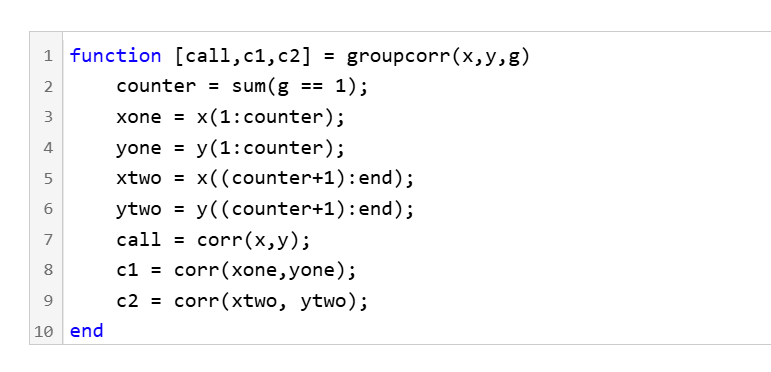
and this is my code
It turns out that "Undefined function 'corr' for input arguments of type 'double'." However, should't the input argument of "corr" be column vectors with single/double values? What's even going on there?
unique treats NaN==NaN as false (as it should) requiring NaN to be replaced if NaN is not considered unique in a particular application. In my application, I am checking uniqueness of table rows using [table_unique,index_unique]=unique(table,"rows","sorted") and would prefer to keep NaN as NaN or missing in table_unique without the overhead of replacing it with a dummy value then replacing it again. Dummy values also have the risk of matching existing values in the table, requiring first finding a dummy value that is not in the table.
uniquen (similar to isequaln) would be more eloquent.
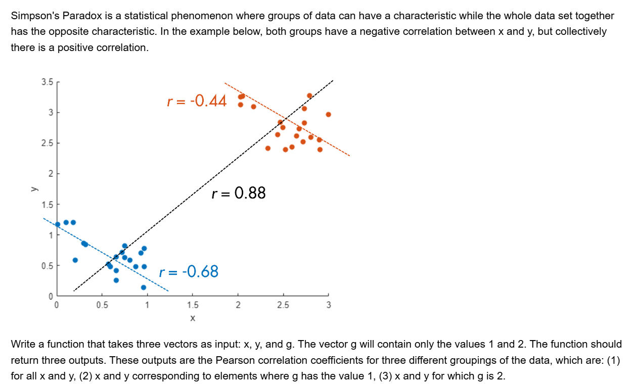
I have an EV model, and I would like to calculate its efficiency, i.e., inverter efficiency, motor efficiency and motor efficiency, and I would also like to draw its efficiency map. What approaches can I use to achieve the said objectives.
For now,
I have connected a power sensor at the battery side, which provides a average power at 0.001 sec.
A three-phase power sensor at inverter's output, which apparantly provides higher power than input.
A rotational power sensor, which also provides averaged mechanical power at 0.001 sec.
Following are the challenges which I am facing.
Higher inverter power.
Negative power as well, depending on the drive cycle especially when torque is negative during deceleration.
I am attaching the EV model. Your guidance on this will be highly appreciated.
So generally I want to be using uifigures over figures. For example I really like the tab group component, which can really help with organizing large numbers of plots in a manageable way. I also really prefer the look of the progress dialog, uialert, confirm, etc. That said, I run into way more bugs using uifigures. I always get a “flicker” in the axes toolbar for example. I also have matlab getting “hung” a lot more often when using uifigures.
So in general, what is recommended? Are uifigures ever going to fully replace traditional figures? Are they going to become more and more robust? Do I need a better GPU to handle graphics better? Just looking for general guidance.
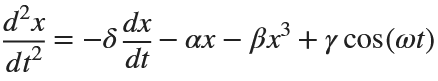
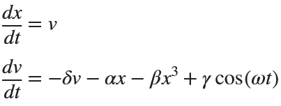
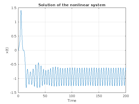
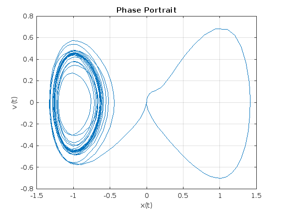
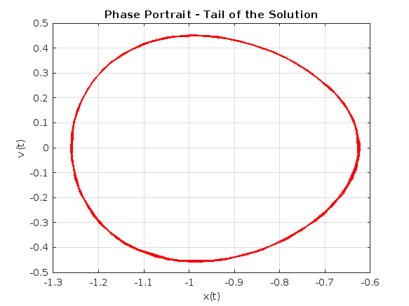
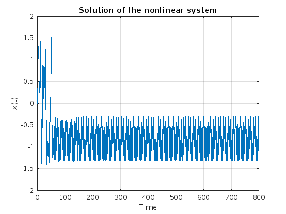
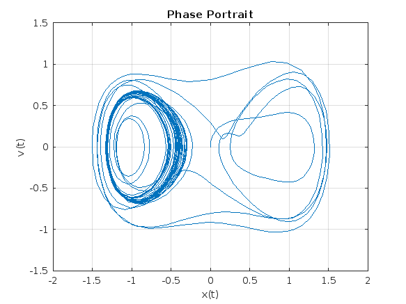
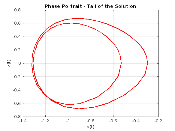
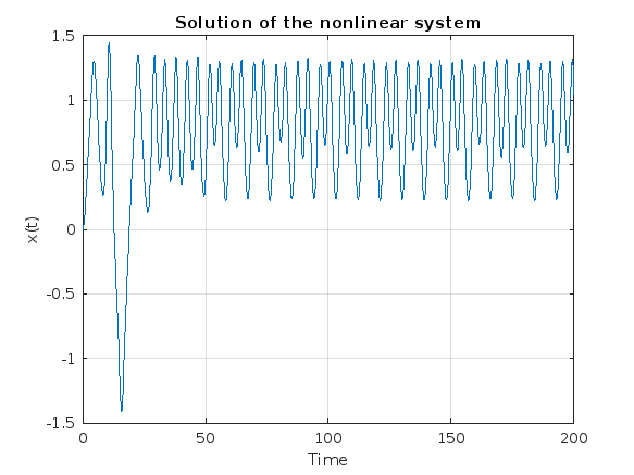
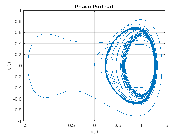
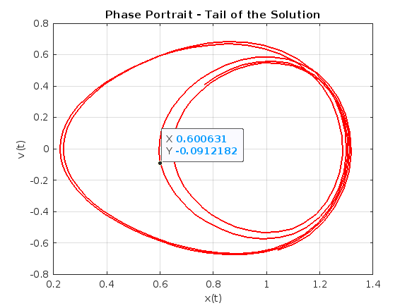
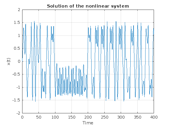
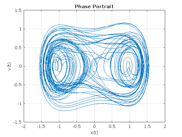
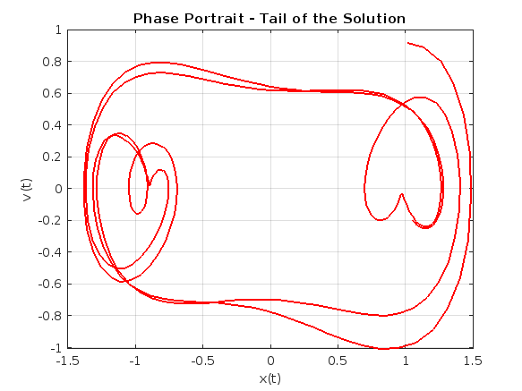
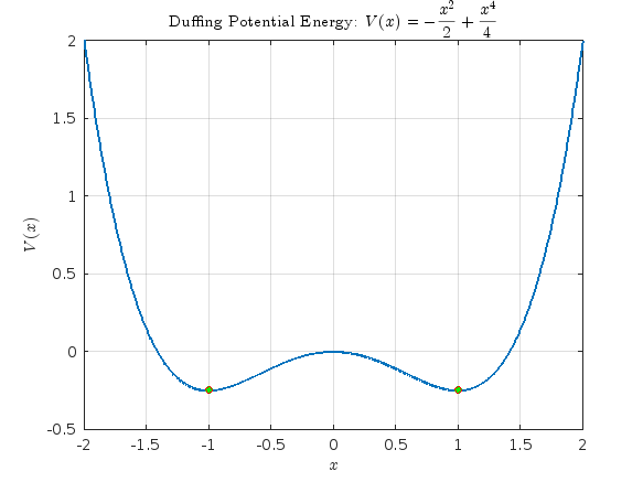
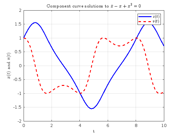
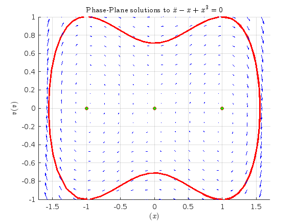
Studying the attached document Duffing Equation from the University of Colorado, I noticed that there is an analysis of The Non-Chaotic Duffing Equation and all the graphs were created with Matlab. And since the code is not given I took the initiative to try to create the same graphs with the following code.
Plotting the Potential Energy and Identifying Extrema
Hello :-) I am interested in reading the book "The finite element method for solid and structural mechanics" online with somebody who is also interested in studying the finite element method particularly its mathematical aspect. I enjoy discussing the book instead of reading it alone. Please if you were interested email me at: student.z.k@hotmail.com Thank you!
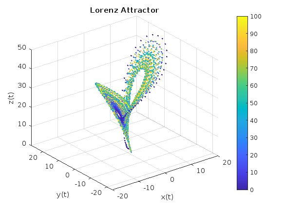
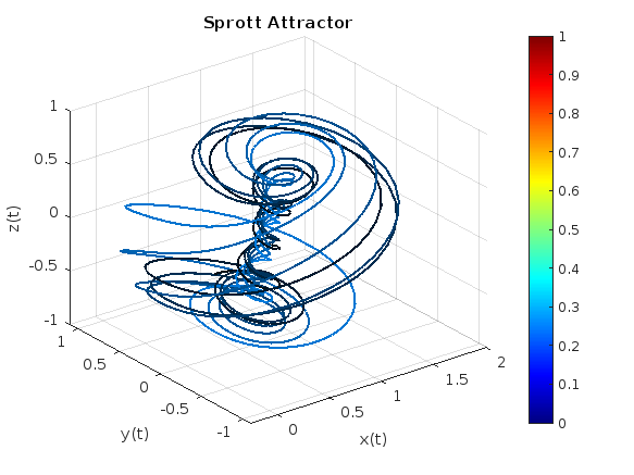
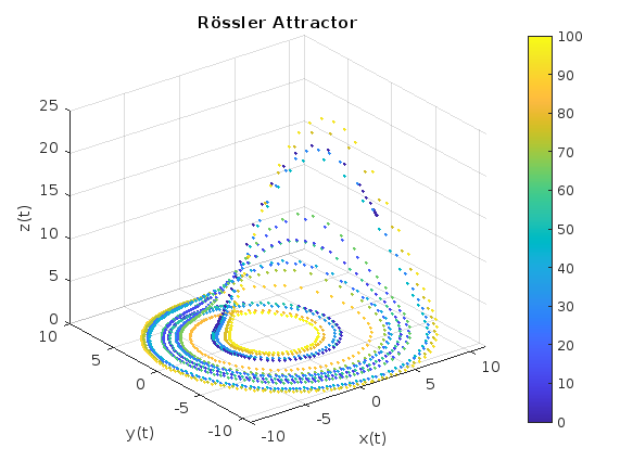
An attractor is called strange if it has a fractal structure, that is if it has non-integer Hausdorff dimension. This is often the case when the dynamics on it are chaotic, but strange nonchaotic attractors also exist. If a strange attractor is chaotic, exhibiting sensitive dependence on initial conditions, then any two arbitrarily close alternative initial points on the attractor, after any of various numbers of iterations, will lead to points that are arbitrarily far apart (subject to the confines of the attractor), and after any of various other numbers of iterations will lead to points that are arbitrarily close together. Thus a dynamic system with a chaotic attractor is locally unstable yet globally stable: once some sequences have entered the attractor, nearby points diverge from one another but never depart from the attractor.
The term strange attractor was coined by David Ruelle and Floris Takens to describe the attractor resulting from a series of bifurcations of a system describing fluid flow. Strange attractors are often differentiable in a few directions, but some are like a Cantor dust, and therefore not differentiable. Strange attractors may also be found in the presence of noise, where they may be shown to support invariant random probability measures of Sinai–Ruelle–Bowen type.
Imagine that the earth is a perfect sphere with a radius of 6371000 meters and there is a rope tightly wrapped around the equator. With one line of MATLAB code determine how much the rope will be lifted above the surface if you cut it and insert a 1 meter segment of rope into it (and then expand the whole rope back into a circle again, of course).
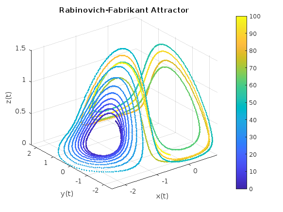
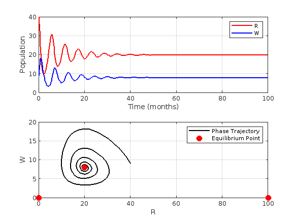
This project discusses predator-prey system, particularly the Lotka-Volterra equations,which model the interaction between two sprecies: prey and predators. Let's solve the Lotka-Volterra equations numerically and visualize the results.% Define parameters
Now, we need to handle a modified version of the Lotka-Volterra equations. These modified equations incorporate logistic growth fot the prey population.
These equations are:
% Define parameters
alpha = 1.0;
K = 100; % Carrying Capacity of the prey population
Does your company or organization require that all your Word Documents and Excel workbooks be labeled with a Microsoft Azure Information Protection label or else they can't be saved? These are the labels that are right below the tool ribbon that apply a category label such as "Public", "Business Use", or "Highly Restricted". If so, you can either
Create and save a "template file" with the desired label and then call copyfile to make a copy of that file and then write your results to the new copy, or
If using Windows you can create and/or open the file using ActiveX and then apply the desired label from your MATLAB program's code.
For #1 you can do
copyfile(templateFileName, newDataFileName);
writematrix(myData, newDataFileName);
If the template has the AIP label applied to it, then the copy will also inherit the same label.
For #2, here is a demo for how to apply the code using ActiveX.
% Test to set the Microsoft Azure Information Protection label on an Excel workbook.
% Save this workbook with the new AIP setting we just created.
Excel.ActiveWorkbook.Save;
% Shut down Excel.
Excel.ActiveWorkbook.Close;
Excel.Quit;
% Excel is now closed down. Delete the variable from the MATLAB workspace.
clear Excel;
% Now check to see if the AIP label has been set
% by opening up the file in Excel and looking at the AIP banner.
winopen(excelFullFileName)
Note that there is a line in there that gets an AIP label from the existing workbook, if there is one at all. If there is not one, you can set one. But to determine what the proper LabelId (that crazy long hexadecimal number) should be, you will probably need to open an existing document that already has the label that you want set (applied to it) and then read that label with this line:
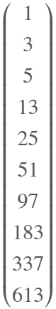
This stems purely from some play on my part. Suppose I asked you to work with the sequence formed as 2*n*F_n + 1, where F_n is the n'th Fibonacci number? Part of me would not be surprised to find there is nothing simple we could do. But, then it costs nothing to try, to see where MATLAB can take me in an explorative sense.
n = sym(0:100).';
Fn = fibonacci(n);
Sn = 2*n.*Fn + 1;
Sn(1:10) % A few elements
ans =
For kicks, I tried asking ChatGPT. Giving it nothing more than the first 20 members of thse sequence as integers, it decided this is a Perrin sequence, and gave me a recurrence relation, but one that is in fact incorrect. Good effort from the Ai, but a fail in the end.
Is there anything I can do? Try null! (Look carefully at the array generated by Toeplitz. It is at least a pretty way to generate the matrix I needed.)
X = toeplitz(Sn,[1,zeros(1,4)]);
rank(X(5:end,:))
ans = 5
Hmm. So there is no linear combination of those columns that yields all zeros, since the resulting matrix was full rank.
X = toeplitz(Sn,[1,zeros(1,5)]);
rank(X(6:end,:))
ans = 5
But if I take it one step further, we see the above matrix is now rank deficient. What does that tell me? It says there is some simple linear combination of the columns of X(6:end,:) that always yields zero. The previous test tells me there is no shorter constant coefficient recurrence releation, using fewer terms.
null(X(6:end,:))
ans =
Let me explain what those coefficients tell me. In fact, they yield a very nice recurrence relation for the sequence S_n, not unlike the original Fibonacci sequence it was based upon.
where the first 5 members of that sequence are given as [1 3 5 13 25]. So a 6 term linear constant coefficient recurrence relation. If it reminds you of the generating relation for the Fibonacci sequence, that is good, because it should. (Remember I started the sequence at n==0, IF you decide to test it out.) We can test it out, like this:
SfunM = memoize(@(N) Sfun(N));
SfunM(25)
ans = 3751251
2*25*fibonacci(sym(25)) + 1
ans =
3751251
And indeed, it works as expected.
function Sn = Sfun(n)
switch n
case 0
Sn = 1;
case 1
Sn = 3;
case 2
Sn = 5;
case 3
Sn = 13;
case 4
Sn = 25;
otherwise
Sn = Sfun(n-5) + Sfun(n-4) - 3*Sfun(n-3) - Sfun(n-2) +3*Sfun(n-1);
end
end
A beauty of this, is I started from nothing but a sequence of integers, derived from an expression where I had no rational expectation of finding a formula, and out drops something pretty. I might call this explorational mathematics.
The next step of course is to go in the other direction. That is, given the derived recurrence relation, if I substitute the formula for S_n in terms of the Fibonacci numbers, can I prove it is valid in general? (Yes.) After all, without some proof, it may fail for n larger than 100. (I'm not sure how much I can cram into a single discussion, so I'll stop at this point for now. If I see interest in the ideas here, I can proceed further. For example, what was I doing with that sequence in the first place? And of course, can I prove the relation is valid? Can I do so using MATLAB?)
(I'll be honest, starting from scratch, I'm not sure it would have been obvious to find that relation, so null was hugely useful here.)
Over the past few weeks, our community has been buzzing with insightful questions, vibrant discussions, and innovative ideas. Whether you're a seasoned expert or a curious beginner, there's something here for everyone to learn and enjoy. Let's take a moment to highlight some of the standout contributions that have sparked interest and inspired many. Dive in and see how you can join the conversation or find solutions to your own challenges!
Oluwadamilola Oke is seeking assistance with a MATLAB code that works on version r2014b but encounters errors on version r2024a. The issue seems to be related to file location or the use of specific commands like movefile. If you have experience with these versions of MATLAB, your expertise could be invaluable.
Yohay has been working on a simulation to measure particle speed and fit it to the Maxwell-Boltzmann distribution. However, the fit isn't aligning perfectly with the data. Yohay has shared the code and histogram data for community members to review and provide suggestions.
Alessandro Livi is toggling between C++ for Arduino Pico and MATLAB App Designer. They suggest an enhancement where typing // for comments in MATLAB automatically converts to %. This small feature could improve the workflow for many users who switch between programming languages.
Athanasios Paraskevopoulos has started an engaging discussion on Gabriel's Horn, a shape with infinite surface area but finite volume. The conversation delves into the mathematical intricacies and integral calculations required to understand this paradoxical shape.
Honzik has brought up an interesting topic about custom fonts for MATLAB. While popular coding fonts handle characters like 0 and O well, they often fail to distinguish between different types of brackets. Honzik suggests that MathWorks could develop a custom font optimized for MATLAB syntax to reduce coding errors.
Guy Rouleau addresses a common error in Simulink models: "Derivative of state '1' in block 'X/Y/Integrator' at time 0.55 is not finite." The blog post explores various tools and methods to diagnose and resolve this issue, making it a valuable read for anyone facing similar challenges.
Guest writer Gianluca Carnielli, featured by Adam Danz, shares insights on creating time-sensitive animations using MATLAB. The article covers controlling the motion of multiple animated objects, organizing data with timetables, and simplifying animations with the retime function. This is a must-read for anyone interested in scientific animations.
Feel free to check out these fascinating contributions and join the discussions! Your input and expertise can make a significant difference in our community.
hello i found the following tools helpful to write matlab programs. copilot.microsoft.com chatgpt.com/gpts gemini.google.com and ai.meta.com. thanks a lot and best wishes.
I have picked the title but don't know which direction to take it. Looking for any and all inspiration. I took the project as it sounded interesting when reading into it, but I'm a satellite novice, and my degree is in electronics.
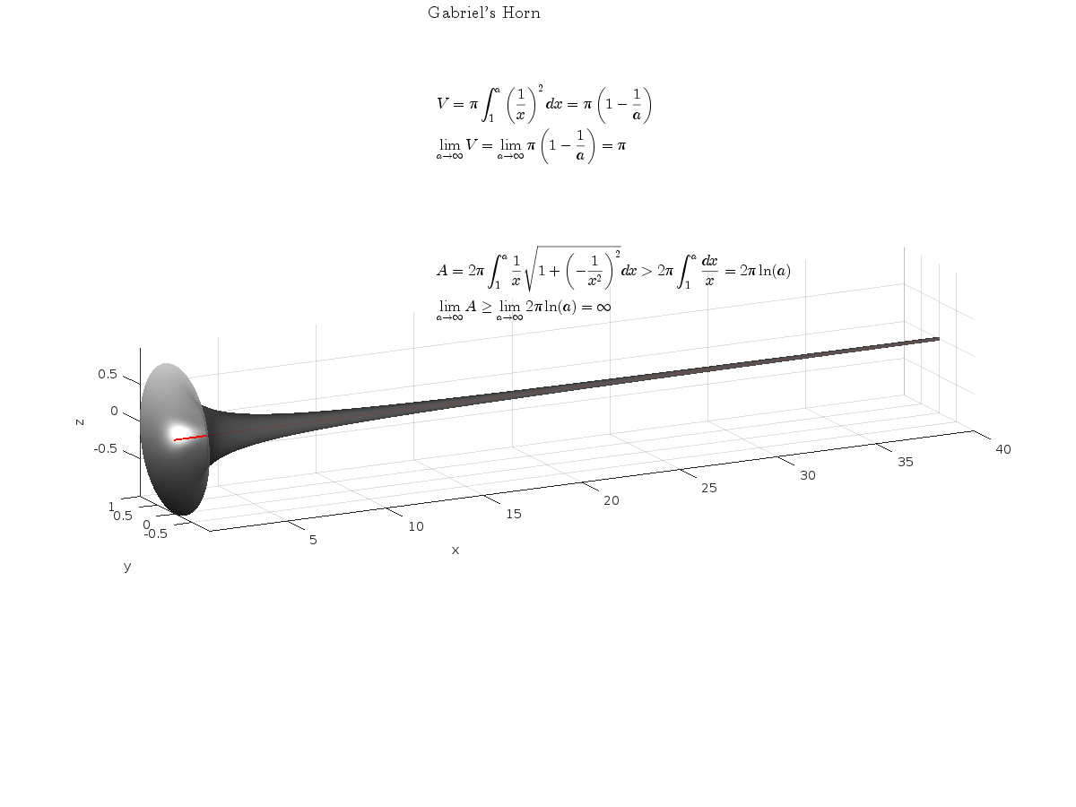
Gabriel's horn is a shape with the paradoxical property that it has infinite surface area, but a finite volume.
Gabriel’s horn is formed by taking the graph of with the domain and rotating it in three dimensions about the axis.
There is a standard formula for calculating the volume of this shape, for a general function .Wwe will just state that the volume of the solid between a and b is:
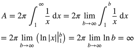
The surface area of the solid is given by:
One other thing we need to consider is that we are trying to find the value of these integrals between 1 and ∞. An integral with a limit of infinity is called an improper integral and we can't evaluate it simply by plugging the value infinity into the normal equation for a definite integral. Instead, we must first calculate the definite integral up to some finite limit b and then calculate the limit of the result as b tends to ∞:
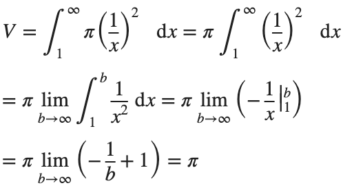
Volume
We can calculate the horn's volume using the volume integral above, so
The total volume of this infinitely long trumpet isπ.
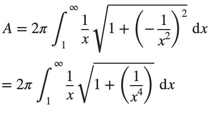
Surface Area
To determine the surface area, we first need the function’s derivative:
Now plug it into the surface area formula and we have:
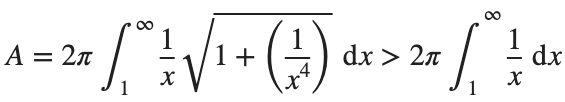
This is an improper integral and it's hard to evaluate, but since in our interval
So, we have :
Now,we evaluate this last integral
So the surface are is infinite.
% Define the function for Gabriel's Horn
gabriels_horn = @(x) 1 ./ x;
% Create a range of x values
x = linspace(1, 40, 4000); % Increase the number of points for better accuracy
y = gabriels_horn(x);
% Create the meshgrid
theta = linspace(0, 2 * pi, 6000); % Increase theta points for a smoother surface
[X, T] = meshgrid(x, theta);
Y = gabriels_horn(X) .* cos(T);
Z = gabriels_horn(X) .* sin(T);
% Plot the surface of Gabriel's Horn
figure('Position', [200, 100, 1200, 900]);
surf(X, Y, Z, 'EdgeColor', 'none', 'FaceAlpha', 0.9);
The properties of this figure were first studied by Italian physicist and mathematician Evangelista Torricelli in the 17th century.
Acknowledgment
I would like to express my sincere gratitude to all those who have supported and inspired me throughout this project.
First and foremost, I would like to thank the mathematician and my esteemed colleague, Stavros Tsalapatis, for inspiring me with the fascinating subject of Gabriel's Horn.
I am also deeply thankful to Mr. @Star Strider for his invaluable assistance in completing the final code.