連続ウェーブレット変換からの周波数局在型の再構成および時間局在型の再構成
阪神淡路大震災データの周波数局在型の Approximation を再構成します。データは 1 Hz でサンプリングされます。CWT から周波数範囲が [0.030, 0.070] Hz の情報を抽出します。
load kobe
Fs = 1;
データの CWT を求めます。
[wt,f] = cwt(kobe,Fs);
地震データを再構成して、信号の平均値を変換後のデータに追加します。
xrec = icwt(wt,[],f,[0.030 0.070],SignalMean=mean(kobe));
元のデータと周波数範囲が [0.030, 0.070] Hz のデータをプロットして比較します。
t = (0:numel(kobe)-1)/60;
tiledlayout(2,1)
nexttile
plot(t,kobe)
grid on
title("Original Data")
nexttile
plot(t,xrec)
grid on
xlabel("Time (mins)")
title("Bandpass Filtered Reconstruction [0.030 0.070] Hz")
![Figure contains 2 axes objects. Axes object 1 with title Original Data contains an object of type line. Axes object 2 with title Bandpass Filtered Reconstruction [0.030 0.070] Hz, xlabel Time (mins) contains an object of type line.](../../examples/wavelet/win64/cwtftdemo_01.png)
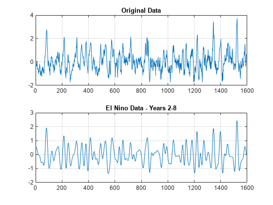
CWT では、周波数の代わりに期間を使用することもできます。毎月サンプリングされるエルニーニョ データを読み込みます。期間を年単位で指定して、CWT を取得します。
load ninoairdata
[cfs,period] = cwt(nino,years(1/12));
2 ~ 8 年目の逆 CWT を求めます。
xrec = icwt(cfs,[],period,[years(2) years(8)]);
再構成されたデータの CWT をプロットします。2 ~ 8 年目の期間に帯域外のエネルギーがないことに注目します。
figure
cwt(xrec,years(1/12))

元のデータと 2 ~ 8 年目について再構成されたデータを比較します。
figure
tiledlayout(2,1)
nexttile
plot(datayear,nino)
grid on
title("Original Data")
nexttile
plot(datayear,xrec)
grid on
title("El Nino Data - Years 2-8")