Stabilize Video Using Optical Flow

This example shows how to stabilize a video that was captured from a jittery platform. One way to stabilize a video is to use keypoint detection and matching to estimate a geometric transform between frames, and use a cumulative accumulation on the transforms to create a smooth camera trajectory. This approach fails when keypoints cannot be reliably detected, such as in textureless regions. This example illustrates a method of video stabilization that works without such a limitation, by using optical flow instead of keypoint detection to match pixels in one video frame to the next. Feature detection based methods are suitable over optical flow in scenarios where faster run-times are important and textureless regions are not an issue. For an example of video stabilization using feature detection, see Stabilize Video Using Image Point Features.

The optical flow based stabilization algorithm involves these steps:

1. Estimate point correspondences between video frames using optical flow.

2. Use point correspondences to estimate the geometric transformation between frames.

3. Warp video frames to obtain a stabilized video.

Read Frames from Video File

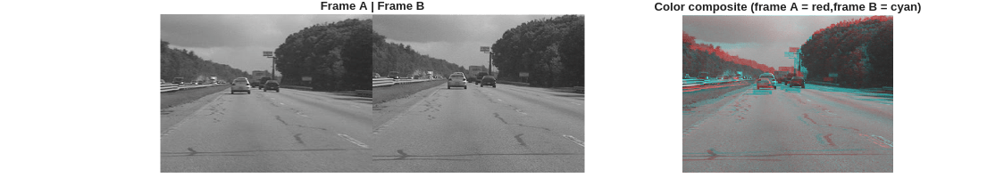
Read the first two frames of a video sequence. Display both frames side by side, then create a red-cyan color composite to illustrate the pixel-wise difference between them. Note, the large vertical and horizontal offset between the two frames.

filename = "shaky_car.avi";
hVideoSrc = VideoReader(filename);

imgA = readFrame(hVideoSrc);
imgA = im2gray(imgA);

imgB = readFrame(hVideoSrc);
imgB = im2gray(imgB);

compositeImg = stereoAnaglyph(imgA,imgB);

figure;
subplot(1,3,[1 2])
montage({imgA,imgB});
title("Frame A | Frame B");

subplot(1,3,3)
imshow(compositeImg);
title("Color composite (frame A = red,frame B = cyan)");
truesize

Select Optical Flow Algorithm

Choose between the Farneback [5] and RAFT [6] optical flow methods. Both algorithms provide dense optical flow at every pixel. Farneback is a classical vision algorithm, does not require a GPU and is faster than RAFT. However, the Farneback algorithm can fail to predict optical flow accurately, particularly in regions of low texture and rapid camera movement. RAFT is a state-of-the-art deep learning model for estimating optical flow that provides highly-accurate results, but requires a GPU for optimal runtime performance.

flowMethod = "Farneback";

switch flowMethod
    case "Farneback"
        flowModel = opticalFlowFarneback;
    case "RAFT"
        flowModel = opticalFlowRAFT;        
end 

Estimate Optical Flow

Compute optical flow between the two frames, and visualize the result.

estimateFlow(flowModel,imgA);
flow = estimateFlow(flowModel,imgB);

Magnify the image and increase the scaling of the plotted optical flow vectors for better visibility.

figure
imshow(imgA, InitialMagnification=250)
hold on
plot(flow,DecimationFactor=[5 5],ScaleFactor=2.0,Color="green");
title("Optical Flow")

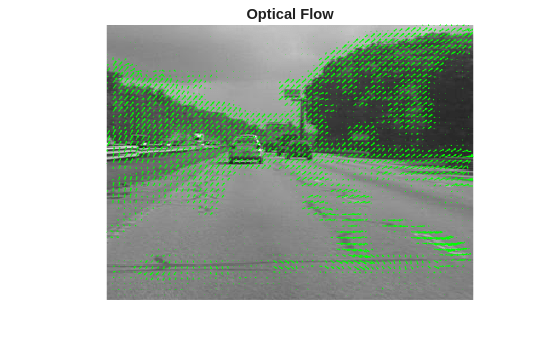
Optical flow vectors are detected correctly on most areas of the image, and most vectors appear to accurately capture the vertical and horizontal motion of the camera jitter. Areas of incorrect flow estimation include patches on the road, which this example addresses when estimating the geometric transformation.

Filter Regions of Invalid Optical Flow

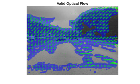
Set the value of minFlowThreshold to discard optical flow vectors with very small magnitudes, as these are likely to have ambiguous orientation. A reasonable default value for this threshold is 1 pixel, which discards flow vectors from regions that have less than 1 pixel of estimated movement. Also discard optical flow vectors that lie outside of the image bounds.

minFlowThreshold = 1;

% Compute target pixel positions in image A from image B
[H,W,~] = size(imgA);
[X1,Y1] = meshgrid(1:W,1:H);
X2 = X1 + flow.Vx;
Y2 = Y1 + flow.Vy;

% Valid optical flow mask
validFlow = X2>=1 & X2<=W & Y2>=1 & Y2<=H & flow.Magnitude > minFlowThreshold;

% Visualize the locations of valid optical flow.
overlayImg = labeloverlay(imgA,validFlow);

figure
imshow(overlayImg, InitialMagnification=250)
hold on
plot(flow,DecimationFactor=[5 5],ScaleFactor=2.0,Color="green");
title("Valid Optical Flow")

Compute Dense Correspondences

Compute densely matched pixels between the two images based on the valid optical flow.

matchedDensePtsA = single([X1(validFlow), Y1(validFlow)]);
matchedDensePtsB = [X2(validFlow), Y2(validFlow)];

Estimate Geometric Transform

A robust estimate of the geometric transformation between the two images can be derived using the M-estimator sample consensus (MSAC) algorithm, a variant of the RANSAC algorithm [1]. The estgeotform2d function implements the MSAC algorithm. This function searches for valid inlier correspondences among a set of point correspondences, and uses the selected correspondences to compute a rigid geometric transformation. This transformation aligns the inliers from the first set of points closely with the inliers from the second set.

tform = estgeotform2d(matchedDensePtsB,matchedDensePtsA,"rigid");
imgBStable = imwarp(imgB,tform,OutputView=imref2d(size(imgB)));

Display the estimated 2-D transform between the two images. This transformation considers 2-D rotation and translation between the two images, without any scaling. Video stabilization generally uses a rigid transform due to better numerical stability, while still being able to capture most of the effects of camera jitter.

disp(tform)

  rigidtform2d with properties:

    Dimensionality: 2
     RotationAngle: -0.6370
       Translation: [-7.9130 8.9640]
                 R: [2×2 single]

                 A: [ 0.9999    0.0111   -7.9130
                     -0.0111    0.9999    8.9640
                           0         0    1.0000]

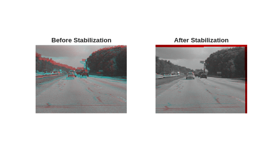
Display the composite image visualizations before and after the stabilization process.

compositeImgStable = stereoAnaglyph(imgA,imgBStable);

figure
subplot(1,2,1)
imshow(compositeImg);
title("Before Stabilization")
subplot(1,2,2)
imshow(compositeImgStable)
title("After Stabilization")

Stabilize on Full Video

Use the previously introduced optical flow stabilization algorithm to smooth a video sequence. At each step, calculate the transformation between the current frames a rigid transform. This combine that transform into a cumulative transformation over a specified number of previous frames.

Initialize Pipeline and Specify Parameter Settings

Reset the video source to the beginning of the file.

hVideoSrc.CurrentTime = 0; 

Reset the optical flow model.

reset(flowModel);

Read the first frame and convert to grayscale.

prevFrame   = readFrame(hVideoSrc);
prevGray    = im2gray(prevFrame);
prevStable  = prevGray;

Initialize the optical flow model with the first frame. The next call to estimateFlow computes the optical flow between the prevGray and the current frame being processed.

estimateFlow(flowModel, prevGray);

Set the threshold in pixels between valid point correspondences when computing the 2-D geometric transform. Larger values cause the RANSAC algorithm to converge faster, at the cost of lower accuracy in the estimation of the transform.

ransacMaxDistance = 4;

Set the maximum number of trials in the RANSAC algorithm for estimating the 2-D geometric transform. Smaller values can speed up the per-frame processing time, at the risk of potentially incorrect results.

ransacMaxNumTrials = 1000;

Process Video Frames

Process video frames one-by-one. This example processes the first 80 frames of the video. To process additional video frames, set the maxFrames variable to your desired value. To smooth the jerky camera motion, when calculating the geometric transform at a frame, this example accumulates the transformations between the previous 10 frames. To modify this cumulative window depending on your data, set the timeWindow variable to your desired value.

frameIndex = 2;
maxFrames = 80;
timeWindow = 10;

figure
allTforms = cell(1,maxFrames);
allTforms{1} = rigidtform2d;

while hasFrame(hVideoSrc) && frameIndex <= maxFrames
    % Read next frame
    frame = readFrame(hVideoSrc);
    frameGray = im2gray(frame);
    
    % Dense optical flow from prevGray to frameGray
    flow = estimateFlow(flowModel, frameGray);

    % Compute target pixel positions in image A from image B
    [H,W,~] = size(frame);
    [X1,Y1] = meshgrid(1:W,1:H);
    X2 = X1 + flow.Vx;
    Y2 = Y1 + flow.Vy;
    
    % Valid optical flow mask
    validFlow = X2>=1 & X2<=W & Y2>=1 & Y2<=H & flow.Magnitude > minFlowThreshold;

    % Compute densely matched pixels between the two images based on valid optical flow
    matchedDensePtsA = single([X1(validFlow), Y1(validFlow)]);
    matchedDensePtsB = [X2(validFlow), Y2(validFlow)];    
    
    % Use RANSAC to estimate a transform from matchedDensePtsA to matchedDensePtsB
    tformFrame = estgeotform2d(matchedDensePtsB,matchedDensePtsA,"rigid",...
        MaxDistance=ransacMaxDistance,MaxNumTrials=ransacMaxNumTrials);

    allTforms{frameIndex} = tformFrame;

    % Accumulate the camera transforms of the last "timeWindow" frames
    windowSize = max(1,frameIndex - timeWindow);
    tformCumulative = rigidtform2d;
    for k = 1:windowSize
        tformCumulative.A = tformCumulative.A * allTforms{frameIndex - k + 1}.A;
    end

    % Warp the current frame using the cumulative transform
    frameStable = imwarp(frameGray,tformCumulative,OutputView=imref2d(size(frameGray)));

    % Display the stabilized frame using red-cyan composites to highlight
    % differences.
    compositeImgRaw = stereoAnaglyph(prevGray,frameGray);
    compositeImgStable = stereoAnaglyph(prevStable,frameStable);
    imViz = cat(2,compositeImgRaw,compositeImgStable);
    
    % Use vision.VideoPlayer to display the video outside of a live script 
imshow(imViz, InitialMagnification=250)
    title("Before Stabilization | After Stabilization")
    drawnow
    
    % Prepare for the next iteration
    prevGray = frameGray;
    prevStable = frameStable;
    frameIndex = frameIndex + 1;
end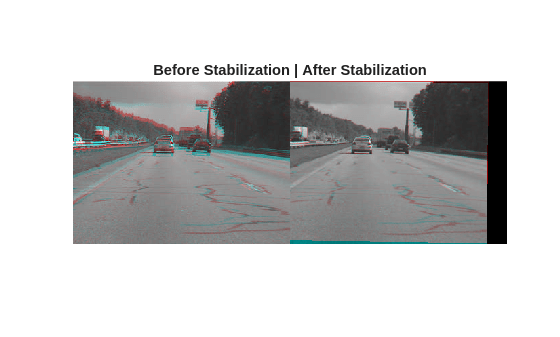

The stabilization approach in this example is able to handle most of the camera jitters, but cannot recover from extremely large motions. More advanced options include using a combination of feature matching and optical flow to determine the transforms between frames, or a more sophisticated method for accumulating the transforms over the video, such as exponentially weighted averaging of the cumulative transforms [9], or performing offline smoothing of the camera trajectory [7][8]. More accurate deep learning-based methods for optical flow, such as opticalFlowRAFT, also yield better quality results, but require a GPU for faster run-times.

References

[1] Tordoff, B; Murray, DW. "Guided sampling and consensus for motion estimation." European Conference in Computer Vision, 2002.

[2] Lee, KY; Chuang, YY; Chen, BY; Ouhyoung, M. "Video Stabilization using Robust Feature Trajectories." International Conference on Computer Vision, 2009.

[3] Litvin, A; Konrad, J; Karl, WC. "Probabilistic video stabilization using Kalman filtering and mosaicking." IS&T/SPIE Symposium on Electronic Imaging, Image and Video Communications and Proc., 2003.

[4] Matsushita, Y; Ofek, E; Tang, X; Shum, HY. "Full-frame Video Stabilization." Microsoft® Research Asia. CVPR 2005.

[5] Farnebäck, G. "Two-Frame Motion Estimation Based on Polynomial Expansion." Scandinavian Conference on Image Analysis*,* 2003.

[6] Teed, Z., & Deng, J. "RAFT: Recurrent All-Pairs Field Transforms for Optical Flow." European Conference in Computer Vision, 2020.

[7] Grundmann, M., Kwatra, V., Essa, I. "Auto-Directed Video Stabilization with Robust L1 Optimal Camera Paths." IEEE Conference on Computer Vision and Pattern Recognition, 2011.

[8] Liu, S. et al. "SteadyFlow: Spatially Smooth Optical Flow for Video Stabilization." IEEE Conference on Computer Vision and Pattern Recognition, 2014.

[9] Battiato, S., Gallo, G., Puglisi, G., & Scellato, S. "SIFT features tracking for video stabilization." International Conference on Image Analysis and Processing, 2007.