Detect Anomaly in Dense 3-D Point Cloud Data Using FPFH Feature Embeddings
This example shows how to detect anomalies in a 3-D dense point cloud data using fast point feature histograms (FPFH) feature embeddings extracted for a single class.
Fast point feature histograms (FPFH) is a feature descriptor used in 3-D point cloud processing to capture local geometric properties around a point, aiding tasks like object recognition and registration. It efficiently represents local surface geometry using histograms of geometric features, such as angles between normals, making it robust to viewpoint changes and partial occlusions. The process involves estimating surface normals, computing simplified point feature histograms (SPFH) for each point by analyzing its neighbors, and aggregating these to form the final FPFH descriptor. This method balances descriptiveness and computational efficiency, making it suitable for real-time applications in computer vision and robotics.
Download Data Set
This example uses the Real3D-AD data set which provides high-resolution 3-D point clouds. The data set comprises a total of 1254 samples that are distributed across 12 distinct categories: Airplane, Car, Candybar, Chicken, Diamond, Duck, Fish, Gemstone, Seahorse, Shell, Starfish, and Toffees.
Download the data set using the helperDownloadReal3dADDataset helper function. The helperDownloadReal3dADDataset helper function is attached to this example as a supporting file.
dataSetDownloadURL = "https://ssd.mathworks.com/supportfiles/vision/data/Real3dadDataset.zip";
dataDir = fullfile(pwd,"Real3dadDataset");
helperDownloadReal3dADDataset(dataSetDownloadURL,dataDir)
You can run this example on any of the classes independently. Select a class to perform the anomaly detection.
className =  "Diamond";
Load Data
Create a fileDatastore object to read and manage the point cloud data from the PCD files in each of the train and test data folders of the specified class.
rootPath = fullfile(dataDir,"data",lower(className));
lidarDataTrain = fileDatastore(fullfile(rootPath,"train"),ReadFcn=@(x)pcread(x));
lidarDataTest = fileDatastore(fullfile(rootPath,"test"),ReadFcn=@(x)pcread(x));
Prepare Data for Training
Specify the first point cloud in the training data set as the target point cloud.
targetPCD = read(lidarDataTrain);
Preprocess Data and Extract FPFH Features
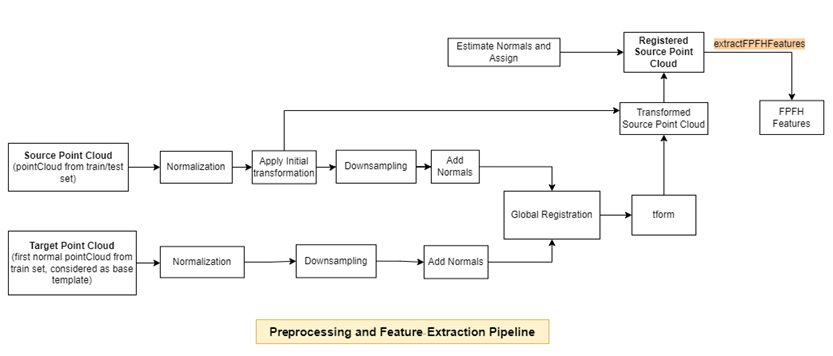
Preprocess each point cloud in the training data set with respect to the target point cloud, and extract FPFH features by using the extractFPFHEmbeddings helper function defined at the end of this example. The extractFPFHEmbeddings function performs these steps.
Normalization — Calculate the centroid of the input point cloud, and shift all the points to origin by using the
normalizePCDhelper function defined at the end of this example.Rigid Transformation — Apply an initial transformation to the input point cloud that essentially performs a coordinate system realignment to roughly align it with the target point cloud, ensuring both are in the same reference frame before global registration. The input point cloud undergoes a rigid transformation, which is useful for an external coarse estimation. This estimation increases the likelihood of finding the correct global alignment and speeds up convergence.
Downsampling — Reduce the number of points in the point cloud and estimate normals for the downsampled point clouds by using the
preprocessPointCloudhelper function defined at the end of this example. Downsampling the point cloud reduces the execution time of subsequent steps. Because you need information from surface normals to extract FPFH features, thepreprocessPointCloudfunction also estimates the normals of the downsampled point clouds.Global Registration — Register the input point cloud to the target point cloud using fast global registration.
FPFH Feature Extraction — Extract FPFH features from the registered input point cloud by using the
extractFPFHFeatures(Lidar Toolbox) function. FPFH features enable you to characterize the local geometry of a point in 3-D space by examining its neighboring points. This process involves analyzing each point along with its nearby neighbors and computing a histogram based on the angles between them. The histogram acts as a fingerprint that encapsulates the local geometry around each point, aiding in identifying corresponding points in the target point cloud.
Track the progress of the preprocessing on and FPFH feature extraction from the training data by using the displayProgress helper function defined at the end of this example.
embedsTrain = [];
numTrainFiles = numel(lidarDataTrain.Files);
reset(lidarDataTrain)

for idx = 1:numTrainFiles
    pcdTrain = read(lidarDataTrain);
    embeds = extractFPFHEmbeddings(pcdTrain,targetPCD);
    embedsTrain = vertcat(embedsTrain,embeds);
    displayProgress(idx,numTrainFiles,"train")
end
The extractFPFHFeatures function returns a memory bank of training features in the variable embedsTrain, which is an N-by-33 embedding matrix for the training data. N is the number of valid points in the input point cloud, each of which has a feature embedding vector of length 33. Observe that the number of points is very large, which could require a long time to further process.
whos embedsTrainProcessing Training Point Cloud 1 of 4 (25.00% complete) Processing Training Point Cloud 2 of 4 (50.00% complete) Processing Training Point Cloud 3 of 4 (75.00% complete) Processing Training Point Cloud 4 of 4 (100.00% complete)
  Name                   Size                 Bytes  Class     Attributes

  embedsTrain      7889811x33            2082910104  double
Subsample Training Embeddings
Apply greedy coreset subsampling to the N-by-33 embedding matrix from the training data to reduce the size of the training feature memory bank, while preserving its distribution, by using the helperComputeApproxGreedyCoresetIndices helper function. The helperComputeApproxGreedyCoresetIndices helper function is attached to this example as a supporting file. Greedy coreset subsampling reduces the computational cost of processing test point clouds during inference and improves efficiency.
Specify the number of samples from which to build the memory bank of training features. Specify verbose as true to display the progress during the selection of coreset indices.
verbose = true;
memorybankSize = 45000;
coresetIndices = helperComputeApproxGreedyCoresetIndices(embedsTrain,memorybankSize,verbose);
45000;
coresetIndices = helperComputeApproxGreedyCoresetIndices(embedsTrain,memorybankSize,verbose);Computing coreset samples Completed 4500 of 45000 Time: Calculating... Completed 9000 of 45000 Time: 03:17 of 12:35 Completed 13500 of 45000 Time: 04:27 of 12:34 Completed 18000 of 45000 Time: 05:36 of 12:33 Completed 22500 of 45000 Time: 06:47 of 12:36 Completed 27000 of 45000 Time: 07:58 of 12:38 Completed 31500 of 45000 Time: 09:08 of 12:39 Completed 36000 of 45000 Time: 10:19 of 12:39 Completed 40500 of 45000 Time: 11:29 of 12:40 Completed 45000 of 45000 Time: 12:40 of 12:40
trainingFeatures = embedsTrain(coresetIndices,:);
Display the extracted FPFH descriptors for the first point from trainingFeatures.
figure
bar(trainingFeatures(1,:),FaceColor=[1 0 0])
title("FPFH Descriptors for First Point of trainingFeatures")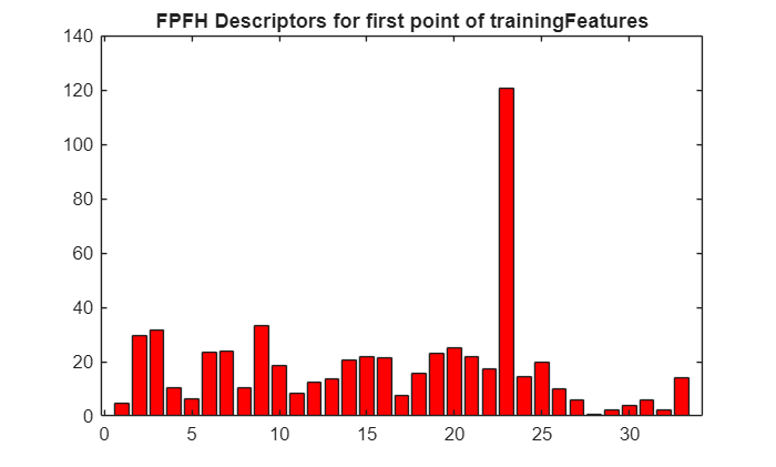
Detect Anomaly in Test Data
Initialize arrays for storing the predicted anomaly scores of points and object-level point clouds.
objectScores = [];
pointScores = [];
Initialize arrays for storing the ground truth labels of points and object-level point clouds in the test data set.
objectLabelsGT = [];
pointLabelsGT = [];
Specify the path for the file containing the ground truth data. The PCD files that have the substring good contain point clouds of normal objects without anomaly. Otherwise, the PCD files contain point clouds of objects that have anomalies. A normal point in a point cloud, has a label of 0, and an anomalous point in a point cloud has a label of 1. In the ground truth file gt.txt, the first three columns contain the location of the points, and the last column represents the label of the point.
gtPath = fullfile(dataDir,"data",lower(className),"gt");
Preprocess each point cloud in the test data set, and extract its FPFH features from the test point cloud by using the extractFPFHEmbeddings helper function. Predict the anomaly scores at both the object and point level by using the predictFPFH helper function defined at the end of this example. The predictFPFH function searches for the nearest neighbors of points from the test point cloud within the subsampled training features space.
reset(lidarDataTest)
testFiles = lidarDataTest.Files;
numTestFiles = numel(testFiles);
if canUseGPU
    trainingFeatures = gpuArray(trainingFeatures);
end

for fileIdx = 1:numTestFiles
    currentTestFile = testFiles(fileIdx);
    [~,fileName,~] = fileparts(currentTestFile);

    if contains(fileName,"good")
        label = 0;
        pcdTest = pcread(string(currentTestFile));
        pointLabel = zeros(size(pcdTest.Location,1),1);
    else
        label = 1;
        gtFile = fullfile(gtPath,string(strcat(fileName,".txt")));
        dataMatrix = readmatrix(gtFile);
        pcdTest = pointCloud(dataMatrix(:,1:3));
        pointLabel = dataMatrix(:,4);
    end

    embedsTestPCD = extractFPFHEmbeddings(pcdTest,targetPCD);
    if canUseGPU
        embedsTestPCD = gpuArray(embedsTestPCD);
    end
    [imageScorePCD,patchScoresPCD] = predictFPFH(trainingFeatures,embedsTestPCD);
    objectScores = [objectScores; imageScorePCD];
    pointScores = [pointScores; patchScoresPCD];

    objectLabelsGT = [objectLabelsGT; label];
    pointLabelsGT = [pointLabelsGT; pointLabel];

    displayProgress(fileIdx,numTestFiles,"test")
end
Processing and Inferencing Test Point Cloud 1 of 100 (1.00% complete)
Processing and Inferencing Test Point Cloud 2 of 100 (2.00% complete)
Processing and Inferencing Test Point Cloud 3 of 100 (3.00% complete)
Processing and Inferencing Test Point Cloud 4 of 100 (4.00% complete)
Processing and Inferencing Test Point Cloud 5 of 100 (5.00% complete)
Processing and Inferencing Test Point Cloud 6 of 100 (6.00% complete)
Processing and Inferencing Test Point Cloud 7 of 100 (7.00% complete)
Processing and Inferencing Test Point Cloud 8 of 100 (8.00% complete)
Processing and Inferencing Test Point Cloud 9 of 100 (9.00% complete)
Processing and Inferencing Test Point Cloud 10 of 100 (10.00% complete)
Processing and Inferencing Test Point Cloud 11 of 100 (11.00% complete)
Processing and Inferencing Test Point Cloud 12 of 100 (12.00% complete)
Processing and Inferencing Test Point Cloud 13 of 100 (13.00% complete)
Processing and Inferencing Test Point Cloud 14 of 100 (14.00% complete)
Processing and Inferencing Test Point Cloud 15 of 100 (15.00% complete)
Processing and Inferencing Test Point Cloud 16 of 100 (16.00% complete)
Processing and Inferencing Test Point Cloud 17 of 100 (17.00% complete)
Processing and Inferencing Test Point Cloud 18 of 100 (18.00% complete)
Processing and Inferencing Test Point Cloud 19 of 100 (19.00% complete)
Processing and Inferencing Test Point Cloud 20 of 100 (20.00% complete)
Processing and Inferencing Test Point Cloud 21 of 100 (21.00% complete)
Processing and Inferencing Test Point Cloud 22 of 100 (22.00% complete)
Processing and Inferencing Test Point Cloud 23 of 100 (23.00% complete)
Processing and Inferencing Test Point Cloud 24 of 100 (24.00% complete)
Processing and Inferencing Test Point Cloud 25 of 100 (25.00% complete)
Processing and Inferencing Test Point Cloud 26 of 100 (26.00% complete)
Processing and Inferencing Test Point Cloud 27 of 100 (27.00% complete)
Processing and Inferencing Test Point Cloud 28 of 100 (28.00% complete)
Processing and Inferencing Test Point Cloud 29 of 100 (29.00% complete)
Processing and Inferencing Test Point Cloud 30 of 100 (30.00% complete)
Processing and Inferencing Test Point Cloud 31 of 100 (31.00% complete)
Processing and Inferencing Test Point Cloud 32 of 100 (32.00% complete)
Processing and Inferencing Test Point Cloud 33 of 100 (33.00% complete)
Processing and Inferencing Test Point Cloud 34 of 100 (34.00% complete)
Processing and Inferencing Test Point Cloud 35 of 100 (35.00% complete)
Processing and Inferencing Test Point Cloud 36 of 100 (36.00% complete)
Processing and Inferencing Test Point Cloud 37 of 100 (37.00% complete)
Processing and Inferencing Test Point Cloud 38 of 100 (38.00% complete)
Processing and Inferencing Test Point Cloud 39 of 100 (39.00% complete)
Processing and Inferencing Test Point Cloud 40 of 100 (40.00% complete)
Processing and Inferencing Test Point Cloud 41 of 100 (41.00% complete)
Processing and Inferencing Test Point Cloud 42 of 100 (42.00% complete)
Processing and Inferencing Test Point Cloud 43 of 100 (43.00% complete)
Processing and Inferencing Test Point Cloud 44 of 100 (44.00% complete)
Processing and Inferencing Test Point Cloud 45 of 100 (45.00% complete)
Processing and Inferencing Test Point Cloud 46 of 100 (46.00% complete)
Processing and Inferencing Test Point Cloud 47 of 100 (47.00% complete)
Processing and Inferencing Test Point Cloud 48 of 100 (48.00% complete)
Processing and Inferencing Test Point Cloud 49 of 100 (49.00% complete)
Processing and Inferencing Test Point Cloud 50 of 100 (50.00% complete)
Processing and Inferencing Test Point Cloud 51 of 100 (51.00% complete)
Processing and Inferencing Test Point Cloud 52 of 100 (52.00% complete)
Processing and Inferencing Test Point Cloud 53 of 100 (53.00% complete)
Processing and Inferencing Test Point Cloud 54 of 100 (54.00% complete)
Processing and Inferencing Test Point Cloud 55 of 100 (55.00% complete)
Processing and Inferencing Test Point Cloud 56 of 100 (56.00% complete)
Processing and Inferencing Test Point Cloud 57 of 100 (57.00% complete)
Processing and Inferencing Test Point Cloud 58 of 100 (58.00% complete)
Processing and Inferencing Test Point Cloud 59 of 100 (59.00% complete)
Processing and Inferencing Test Point Cloud 60 of 100 (60.00% complete)
Processing and Inferencing Test Point Cloud 61 of 100 (61.00% complete)
Processing and Inferencing Test Point Cloud 62 of 100 (62.00% complete)
Processing and Inferencing Test Point Cloud 63 of 100 (63.00% complete)
Processing and Inferencing Test Point Cloud 64 of 100 (64.00% complete)
Processing and Inferencing Test Point Cloud 65 of 100 (65.00% complete)
Processing and Inferencing Test Point Cloud 66 of 100 (66.00% complete)
Processing and Inferencing Test Point Cloud 67 of 100 (67.00% complete)
Processing and Inferencing Test Point Cloud 68 of 100 (68.00% complete)
Processing and Inferencing Test Point Cloud 69 of 100 (69.00% complete)
Processing and Inferencing Test Point Cloud 70 of 100 (70.00% complete)
Processing and Inferencing Test Point Cloud 71 of 100 (71.00% complete)
Processing and Inferencing Test Point Cloud 72 of 100 (72.00% complete)
Processing and Inferencing Test Point Cloud 73 of 100 (73.00% complete)
Processing and Inferencing Test Point Cloud 74 of 100 (74.00% complete)
Processing and Inferencing Test Point Cloud 75 of 100 (75.00% complete)
Processing and Inferencing Test Point Cloud 76 of 100 (76.00% complete)
Processing and Inferencing Test Point Cloud 77 of 100 (77.00% complete)
Processing and Inferencing Test Point Cloud 78 of 100 (78.00% complete)
Processing and Inferencing Test Point Cloud 79 of 100 (79.00% complete)
Processing and Inferencing Test Point Cloud 80 of 100 (80.00% complete)
Processing and Inferencing Test Point Cloud 81 of 100 (81.00% complete)
Processing and Inferencing Test Point Cloud 82 of 100 (82.00% complete)
Processing and Inferencing Test Point Cloud 83 of 100 (83.00% complete)
Processing and Inferencing Test Point Cloud 84 of 100 (84.00% complete)
Processing and Inferencing Test Point Cloud 85 of 100 (85.00% complete)
Processing and Inferencing Test Point Cloud 86 of 100 (86.00% complete)
Processing and Inferencing Test Point Cloud 87 of 100 (87.00% complete)
Processing and Inferencing Test Point Cloud 88 of 100 (88.00% complete)
Processing and Inferencing Test Point Cloud 89 of 100 (89.00% complete)
Processing and Inferencing Test Point Cloud 90 of 100 (90.00% complete)
Processing and Inferencing Test Point Cloud 91 of 100 (91.00% complete)
Processing and Inferencing Test Point Cloud 92 of 100 (92.00% complete)
Processing and Inferencing Test Point Cloud 93 of 100 (93.00% complete)
Processing and Inferencing Test Point Cloud 94 of 100 (94.00% complete)
Processing and Inferencing Test Point Cloud 95 of 100 (95.00% complete)
Processing and Inferencing Test Point Cloud 96 of 100 (96.00% complete)
Processing and Inferencing Test Point Cloud 97 of 100 (97.00% complete)
Processing and Inferencing Test Point Cloud 98 of 100 (98.00% complete)
Processing and Inferencing Test Point Cloud 99 of 100 (99.00% complete)
Processing and Inferencing Test Point Cloud 100 of 100 (100.00% complete)
Perform min-max normalization across the observed objectScores so that 0 represents the lowest anomaly score observed for a point cloud in the test set and 1 represents the highest observed anomaly score.
mini = min(objectScores,[],"all");
maxi = max(objectScores,[],"all");
objectScores = rescale(objectScores,InputMin=mini,InputMax=maxi);
mini = min(pointScores,[],"all");
maxi = max(pointScores,[],"all");
pointScores = rescale(pointScores,InputMin=mini,InputMax=maxi);
Evaluate Model on Test Data
Evaluate the model on the anomaly scores of points and object-level point clouds.
Compute AUC Score
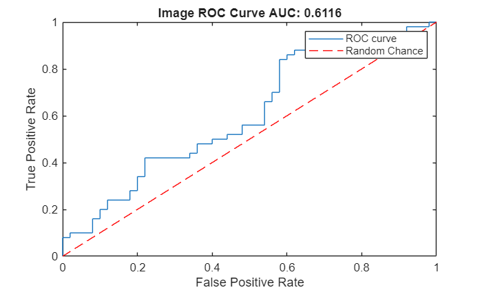
Create an ROC curve by using the perfcurve (Statistics and Machine Learning Toolbox) function. The solid blue line represents the ROC curve. The red dashed line represents a random classifier corresponding to a 50% success rate. Display the area under the ROC curve (AUC) metric for the test data set in the title of the figure. A perfect classifier has an ROC curve with a maximum AUC of 1.
Object-Level ROC Curve
Compute the area under the ROC curve for object-level anomaly scores in the test data set.
[xroc,yroc,~,aurocObject] = perfcurve(objectLabelsGT,objectScores,1);

figure
lroc = plot(xroc,yroc);
hold on
lchance = plot([0 1],[0 1],"r--");
hold off
xlabel("False Positive Rate")
ylabel("True Positive Rate")
title("Image ROC Curve AUC: "+num2str(aurocObject))
legend([lroc lchance],"ROC curve","Random Chance")
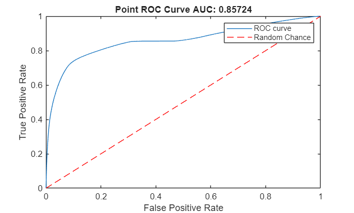
Point-Level ROC Curve
Compute the area under the ROC curve for the anomaly scores of points in the point clouds in the test data set.
[xroc,yroc,~,aurocPoint] = perfcurve(pointLabelsGT,pointScores,1);
figure
lroc = plot(xroc,yroc);
hold on
lchance = plot([0 1],[0 1],"r--");
hold off
xlabel("False Positive Rate")
ylabel("True Positive Rate")
title("Point ROC Curve AUC: "+num2str(aurocPoint))
legend([lroc lchance],"ROC curve","Random Chance")
Compute AUPRC Score
In anomaly detection, the area under the precision-recall curve (AUPRC) measures how well a model identifies rare anomalies among mostly normal data. An AUPRC closer to 1 indicates that the model is better at detecting anomalies with fewer false positives. An AUPRC closer to 0 indicates poor performance, often missing anomalies or misclassifying normal points as anomalies.
Object-Level AUPRC
Compute the AUPRC for object-level anomaly scores in the test data set.
[recall,precision,~,~,~] = perfcurve(objectLabelsGT,objectScores,1,xCrit="reca",yCrit="prec");
precision(isnan(precision)) = 0;
recall(isnan(recall)) = 0;
auprObject = trapz(recall,precision);
display(auprObject)
averagePrecisionObject =

    0.6044
Point-Level AUPRC
Compute the AUPRC for anomaly scores of points in the point clouds in the test data set.
[recall,precision,~,~,~] = perfcurve(pointLabelsGT,pointScores,1,xCrit="reca",yCrit="prec");
precision(isnan(precision)) = 0;
recall(isnan(recall)) = 0;
auprPoint = trapz(recall,precision);
display(auprPoint)
averagePrecisionPoint =

    0.3445
Visualize Anomaly Map
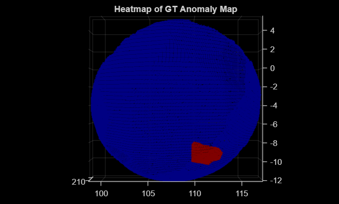
The labels of each point in a point cloud make up the label mask of the point cloud. Read a sample test point cloud, and create a heatmap of its ground truth label mask by using the getHeatmapFromMask helper function defined at the end of this example. Display the sample test point cloud with the ground truth label mask overlaid on it as a heatmap.
dataMatrix = readmatrix(fullfile(dataDir,"data",lower(className),"gt","370_bulge_cut.txt"));
pcdTestSample = pointCloud(dataMatrix(:,1:3));
gtMaskPCDTest = dataMatrix(:,4);
heatmapGT = getHeatmapFromMask(gtMaskPCDTest);
figure
pcdTestSample.Color = gather(heatmapGT);
pcshow(pcdTestSample,ViewPlane="XY")
title("Heatmap of GT Anomaly Map")
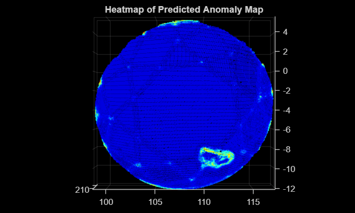
Predict the anomaly score and label mask for the sample test point cloud by using the predictScoreAndMaskForSinglePCD helper function defined at the end of this example. Create a heatmap of the predicted label mask by using the getHeatmapFromMask helper function. Visualize the predicted label mask as a heatmap overlaid on the sample test point cloud data.
[scorePCDTestSample,maskPCDTestSample] = predictScoreAndMaskForSinglePCD(trainingFeatures,pcdTestSample,targetPCD);
heatmapPred = getHeatmapFromMask(maskPCDTestSample);
figure
pcdTestSample.Color = gather(heatmapPred);
pcshow(pcdTestSample,ViewPlane="XY")
title("Heatmap of Predicted Anomaly Map")
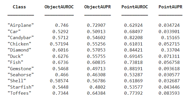
Predict Anomaly Scores for All Classes
You can compute the object-level and point-level AUC and AUPRC scores for all 12 classes in the data set for a specified memory bank size. Specify the className and memorybankSize values to use to compute the scores. This table describes the object-level and point-level AUC and AUPRC scores for all 12 classes for a memory bank size of 25,000.
References
[1] Liu, Jiaqi, Guoyang Xie, Ruitao Chen, Xinpeng Li, Jinbao Wang, Yong Liu, Chengjie Wang, Feng Zheng. "Real3D-AD: A Dataset of Point Cloud Anomaly Detection." Advances in Neural Information Processing Systems 36. February 13, 2024. https://doi.org/10.48550/arXiv.2309.13226.
Supporting Functions
function embeds = extractFPFHEmbeddings(sourceData,targetData)
    rng(42) % Fix a seed

    % Normalize the source and target point clouds
    sourceDataNorm = normalizePCD(sourceData);
    targetDataNorm = normalizePCD(targetData);

    % Define the initial rigid transformation matrix
    transInit = [0.0  0.0  1.0  0.0;
                 1.0  0.0  0.0  0.0;
                 0.0  1.0  0.0  0.0;
                 0.0  0.0  0.0  1.0];
    tform = rigidtform3d(transInit);
    % Apply initial transformation to approximately align the source point cloud
    sourceTransformed = pctransform(sourceDataNorm,tform);

    % Preprocess the source and target point clouds by downsampling and
    % assigning normals
    gridSize = 0.5;
    sourceDownSampled = preprocessPointCloud(sourceTransformed,gridSize);
    targetDownSampled = preprocessPointCloud(targetDataNorm,gridSize);

    % Perform global registration on downsampled point clouds
    maxIterations = 100;
    [rotation,translation,~] = fastGlobalRegistration(sourceDownSampled.Location, ...
        targetDownSampled.Location,sourceDownSampled.Normal,targetDownSampled.Normal,gridSize, ...
        uint16(maxIterations));
    tformReg = rigidtform3d(rotation,translation);

    % Apply registered tform to source point cloud
    sourceReg = pctransform(sourceTransformed,tformReg);

    % Estimate normals
    maxNN = 30; % Maximum number of nearest neighbors
    normals = pcnormals(sourceReg,maxNN);
    % Assign the estimated normals to the point cloud
    sourceReg.Normal = normals;

    % Extract the FPFH features
    radiusFeatures = gridSize*5;
    embeds = extractFPFHFeatures(sourceReg,Radius=radiusFeatures,NumNeighbors=100);
end


function newPtCloud = normalizePCD(ptCloud)
    % Calculate the centroid of the point cloud
    center = mean(ptCloud.Location,1);

    % Shift the point cloud to center it at the origin
    newXYZPoints = ptCloud.Location - center;
    newPtCloud = pointCloud(newXYZPoints);
end


function pcdDown = preprocessPointCloud(pcd,voxelSize)
    % Downsample the input point cloud
    pcdDown = pcdownsample(pcd,"gridNearest",voxelSize);

    maxNN = 30; % Maximum number of nearest neighbors
    normals = pcnormals(pcdDown,maxNN);

    % Assign the estimated normals to the point cloud
    pcdDown.Normal = normals;
end

function displayProgress(idx,numFiles,str)
    progress = (idx/numFiles)*100;
    if strcmp(str,"train")
        fprintf("Processing Training Point Cloud %d of %d (%.2f%% complete)\n",idx,numFiles,progress)
    else
        fprintf("Processing and Inferencing Test Point Cloud %d of %d (%.2f%% complete)\n",idx,numFiles,progress)
    end
end

function [imageScores,patchScores] = predictFPFH(trainingFeatures,embeddingsIn)
    rng("default") % Fix a seed
    knnDist = pdist2(trainingFeatures,embeddingsIn,"euclidean",Smallest=1);
    knnDist = knnDist';

    maxDist = max(knnDist(:,1));

    imageScores =  maxDist;
    patchScores = knnDist;
end

function heatmap = getHeatmapFromMask(maskIn)
    % Convert to an indexed image with 256 levels (0-255)
    indexedImage = double(maskIn)*255;
    % Apply the jet colormap
    colormapJet = jet(256);
    heatmap = ind2rgb(uint8(indexedImage),colormapJet);

    % Remove any singleton dimensions
    heatmap = squeeze(heatmap);
end

function [score,mask] = predictScoreAndMaskForSinglePCD(trainingFeatures,pcdTestSample,basicTemplatePCD)
    embedsTestPCDSample = extractFPFHEmbeddings(pcdTestSample,basicTemplatePCD);
    if canUseGPU
        trainingFeatures = gpuArray(trainingFeatures);
        embedsTestPCDSample = gpuArray(embedsTestPCDSample);
    end
    [score,mask] = predictFPFH(trainingFeatures,embedsTestPCDSample);

    mini = min(mask,[],"all");
    maxi = max(mask,[],"all");
    mask = rescale(mask,InputMin=mini,InputMax=maxi);
end
See Also
pointCloud | extractFPFHFeatures (Lidar Toolbox)