Optimization Toolbox ソルバーによる記号数学の使用

この例では次を使用します。

この例では、Symbolic Math Toolbox™ の関数 jacobian および matlabFunction を使用して、解析的な導関数を最適化ソルバーに与える方法を説明します。一般に、Optimization Toolbox™ ソルバーの精度と効率は、目的関数と制約関数の勾配とヘッシアンが与えられた場合に向上します。

問題ベースの最適化では、勾配を自動的に計算して使用できます。Optimization Toolbox の自動微分 (Optimization Toolbox)を参照してください。自動微分を使用した問題ベースの例については、最適化変数を使用した静電学における制約付き非線形最適化 (Optimization Toolbox)を参照してください。

最適化関数でシンボリックな計算を使用する際は、以下のことを考慮しなければなりません。

最適化の目的関数と制約関数は、x のように、ベクトルで定義する必要があります。ただし、シンボリック変数はベクトル値ではなく、スカラーまたは複素数値です。このため、ベクトルとスカラー間の変換が必要です。
最適化の勾配と、場合によりますがヘッシアンは、目的関数または制約関数の本体内で計算されることになっています。これは、シンボリックな勾配またはヘッシアンを、目的関数または制約関数ファイル、あるいは関数ハンドル内の適切な位置に配置する必要があることを意味します。
勾配とヘッシアンのシンボリックな計算には、時間がかかることがあります。このため、ソルバーの実行中に呼び出すために、この計算を一度だけ実行し、matlabFunction を使用してコードを生成する必要があります。
関数 subs を使用したシンボリック式の評価には、時間がかかります。matlabFunction を使用した方が、はるかに効率的です。
matlabFunction は、入力ベクトルの方向に依存するコードを生成します。fmincon は列ベクトルを含む目的関数を呼び出すため、シンボリック変数の列ベクトルを含む matlabFunction を呼び出す際は注意しなければなりません。

第 1 の例:ヘッシアンを使用した制約なし最小化

最小化する目的関数は以下のとおりです。

$f (x_{1}, x_{2}) = \log (1 + 3 {(x_{2} - (x_{1}^{3} - x_{1}))}^{2} + (x_{1} - 4 / 3)^{2}) .$

この関数は正であり、x1 = 4/3, x2 =(4/3)^3 - 4/3 = 1.0370... において固有の最小値ゼロに到達します。

独立変数を x1 および x2 として記述します。その理由は、この形式で、独立変数をシンボリック変数として使用できるからです。ベクトル x の成分としては、x(1) および x(2) と記述されます。この関数は、次のプロットで示したように、曲がりくねった谷を持っています。

syms x1 x2 real
x = [x1;x2]; % column vector of symbolic variables
f = log(1 + 3*(x2 - (x1^3 - x1))^2 + (x1 - 4/3)^2)

f = 
 $\log ({(x_{1} - \frac{4}{3})}^{2} + 3 {(- {x_{1}}^{3} + x_{1} + x_{2})}^{2} + 1)$

fsurf(f,[-2 2],'ShowContours','on')
view(127,38)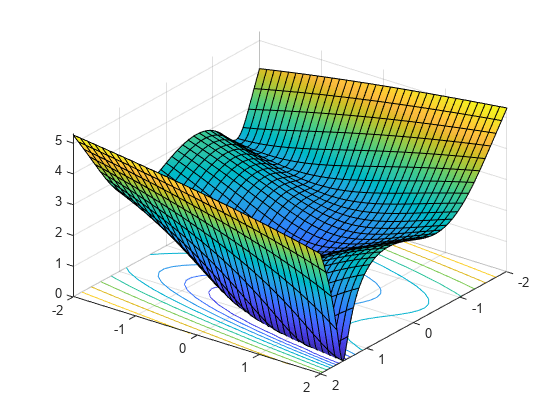

Figure contains an axes object. The axes object contains an object of type functionsurface.

f の勾配とヘッシアンを計算します。

gradf = jacobian(f,x).' % column gradf

gradf = 
 $\begin{array}{l} (\begin{array}{c} - \frac{6 (3 {x_{1}}^{2} - 1) (- {x_{1}}^{3} + x_{1} + x_{2}) - 2 x_{1} + \frac{8}{3}}{σ_{1}} \\ \frac{- 6 {x_{1}}^{3} + 6 x_{1} + 6 x_{2}}{σ_{1}} \end{array}) \\ where \\ σ_{1} = {(x_{1} - \frac{4}{3})}^{2} + 3 {(- {x_{1}}^{3} + x_{1} + x_{2})}^{2} + 1 \end{array}$

hessf = jacobian(gradf,x)

hessf = 
 $\begin{array}{l} (\begin{array}{c} \frac{6 {(3 {x_{1}}^{2} - 1)}^{2} - 36 x_{1} (- {x_{1}}^{3} + x_{1} + x_{2}) + 2}{σ_{2}} - \frac{{σ_{3}}^{2}}{{σ_{2}}^{2}} & σ_{1} \\ σ_{1} & \frac{6}{σ_{2}} - \frac{{(- 6 {x_{1}}^{3} + 6 x_{1} + 6 x_{2})}^{2}}{{σ_{2}}^{2}} \end{array}) \\ where \\ σ_{1} = \frac{(- 6 {x_{1}}^{3} + 6 x_{1} + 6 x_{2}) σ_{3}}{{σ_{2}}^{2}} - \frac{18 {x_{1}}^{2} - 6}{σ_{2}} \\ σ_{2} = {(x_{1} - \frac{4}{3})}^{2} + 3 {(- {x_{1}}^{3} + x_{1} + x_{2})}^{2} + 1 \\ σ_{3} = 6 (3 {x_{1}}^{2} - 1) (- {x_{1}}^{3} + x_{1} + x_{2}) - 2 x_{1} + \frac{8}{3} \end{array}$

fminunc ソルバーには、ベクトル x を渡し、SpecifyObjectiveGradient オプションを true に、HessianFcn オプションを 'objective' に設定して、次の 3 つの出力のリストを与えます。[f(x),gradf(x),hessf(x)]。

matlabFunction は、3 つの入力のリストから 3 つの出力のこのリストを正確に生成します。matlabFunction はさらに、vars オプションを使用してベクトル入力を受け取ります。

fh = matlabFunction(f,gradf,hessf,'vars',{x});

点 [-1,2] から始めて、最小化問題を解きます。

options = optimoptions('fminunc', ...
    'SpecifyObjectiveGradient', true, ...
    'HessianFcn', 'objective', ...
    'Algorithm','trust-region', ...
    'Display','final');
[xfinal,fval,exitflag,output] = fminunc(fh,[-1;2],options)

Local minimum possible.

fminunc stopped because the final change in function value relative to 
its initial value is less than the value of the function tolerance.

xfinal = 2×1

    1.3333
    1.0370

fval = 7.6623e-12

exitflag = 3

output = struct with fields:
         iterations: 14
          funcCount: 15
           stepsize: 0.0027
       cgiterations: 11
      firstorderopt: 3.4391e-05
          algorithm: 'trust-region'
            message: 'Local minimum possible....'
    constrviolation: []

これを、勾配またはヘッセ情報を使用しない場合の反復の回数と比較します。これには 'quasi-newton' アルゴリズムが必要になります。

options = optimoptions('fminunc','Display','final','Algorithm','quasi-newton');
fh2 = matlabFunction(f,'vars',{x}); 
% fh2 = objective with no gradient or Hessian
[xfinal,fval,exitflag,output2] = fminunc(fh2,[-1;2],options)

Local minimum found.

Optimization completed because the size of the gradient is less than
the value of the optimality tolerance.

xfinal = 2×1

    1.3333
    1.0371

fval = 2.1985e-11

exitflag = 1

output2 = struct with fields:
       iterations: 18
        funcCount: 81
         stepsize: 2.1164e-04
     lssteplength: 1
    firstorderopt: 2.4587e-06
        algorithm: 'quasi-newton'
          message: 'Local minimum found....'

反復回数は、勾配とヘッシアンを使用した場合が少なく、関数評価の回数が激減します。

sprintf(['There were %d iterations using gradient' ...
    ' and Hessian, but %d without them.'], ...
    output.iterations,output2.iterations)

ans = 
'There were 14 iterations using gradient and Hessian, but 18 without them.'

sprintf(['There were %d function evaluations using gradient' ...
    ' and Hessian, but %d without them.'], ...
    output.funcCount,output2.funcCount)

ans = 
'There were 15 function evaluations using gradient and Hessian, but 81 without them.'

第 2 の例:fmincon の内点法アルゴリズムを使用した制約付き最小化

第 1 の例と同じ目的関数と開始値を検討しますが、第 2 の例には 2 つの非線形制約があります。

$5 \sinh (x_{2} / 5) \geq x_{1}^{4}$

$5 \tanh (x_{1} / 5) \geq x_{2}^{2} - 1 .$

この制約により、最適化が大域的最小点 [1.333,1.037] から離されます。この 2 つの制約を視覚化します。

[X,Y] = meshgrid(-2:.01:3);
Z = (5*sinh(Y./5) >= X.^4); 
% Z=1 where the first constraint is satisfied, Z=0 otherwise
Z = Z+ 2*(5*tanh(X./5) >= Y.^2 - 1); 
% Z=2 where the second is satisfied, Z=3 where both are
surf(X,Y,Z,'LineStyle','none');
fig = gcf;
fig.Color = 'w'; % white background
view(0,90)
hold on
plot3(.4396, .0373, 4,'o','MarkerEdgeColor','r','MarkerSize',8); 
% best point
xlabel('x')
ylabel('y')
hold off

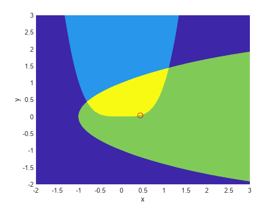
Figure contains an axes object. The axes object with xlabel x, ylabel y contains 2 objects of type surface, line. One or more of the lines displays its values using only markers

最適点の周囲に小さい赤色の円をプロットしました。

実行可能領域全体にわたって目的関数のプロットがあります。これは両方の制約を満たす領域であり、最適点の周囲の小さい赤色の円と共に濃い赤色で示されています。

W = log(1 + 3*(Y - (X.^3 - X)).^2 + (X - 4/3).^2); 
% W = the objective function
W(Z < 3) = nan; % plot only where the constraints are satisfied
surf(X,Y,W,'LineStyle','none');
view(68,20)
hold on
plot3(.4396, .0373, .8152,'o','MarkerEdgeColor','r', ...
    'MarkerSize',8); % best point
xlabel('x')
ylabel('y')
zlabel('z')
hold off

Figure contains an axes object. The axes object with xlabel x, ylabel y contains 2 objects of type surface, line. One or more of the lines displays its values using only markers

非線形制約は、c(x) <= 0 という形式で記述しなければなりません。matlabFunction を使用して、すべてのシンボリック制約とその導関数を計算し、関数ハンドルに配置します。

これらの制約の勾配は、列ベクトルにする必要があります。これらは、各列が 1 つの制約関数の勾配を表すような行列として目的関数に配置しなければなりません。これは jacobian によって生成される形式の転置行列であるため、以下では転置行列を求めます。

非線形制約を関数ハンドルに配置します。fmincon は、非線形制約と勾配が [c ceq gradc gradceq] という順序で出力されると想定します。非線形等式制約が存在しないため、ceq と gradceq として [] を出力します。

c1 = x1^4 - 5*sinh(x2/5);
c2 = x2^2 - 5*tanh(x1/5) - 1;
c = [c1 c2];
gradc = jacobian(c,x).'; % transpose to put in correct form
constraint = matlabFunction(c,[],gradc,[],'vars',{x});

内点法アルゴリズムでは、ヘッセ関数を、目的関数の一部ではなく別個の関数として記述する必要があります。これは、非線形制約関数でこれらの制約をヘッシアンに含める必要があるからです。内点法アルゴリズムのヘッシアンは、ラグランジュ関数のヘッシアンです。詳細は、ユーザーガイドを参照してください。

ヘッセ関数には、2 つの入力引数を指定します。正のベクトル x とラグランジュ乗数構造体 lambda です。非線形制約に使用する lambda 構造体の部分は、lambda.ineqnonlin と lambda.eqnonlin です。現在の制約の場合は、非線形等式が存在しないため、lambda.ineqnonlin(1) と lambda.ineqnonlin(2) という 2 つの乗数を使用します。

第 1 の例では、目的関数のヘッシアンを計算しました。ここでは、2 つの制約関数のヘッシアンを計算し、matlabFunction で関数ハンドルバージョンを作成します。

hessc1 = jacobian(gradc(:,1),x); % constraint = first c column
hessc2 = jacobian(gradc(:,2),x);

hessfh = matlabFunction(hessf,'vars',{x});
hessc1h = matlabFunction(hessc1,'vars',{x});
hessc2h = matlabFunction(hessc2,'vars',{x});

最終的なヘッシアンを作成するために、3 つのヘッシアンを統合し、適切なラグランジュ乗数を制約関数に追加します。

myhess = @(x,lambda)(hessfh(x) + ...
    lambda.ineqnonlin(1)*hessc1h(x) + ...
    lambda.ineqnonlin(2)*hessc2h(x));

内点法アルゴリズム、勾配、およびヘッシアンを使用するためのオプションを設定し、目的関数が目的と勾配の両方を返すようにした後、ソルバーを実行します。

options = optimoptions('fmincon', ...
    'Algorithm','interior-point', ...
    'SpecifyObjectiveGradient',true, ...
    'SpecifyConstraintGradient',true, ...
    'HessianFcn',myhess, ...
    'Display','final');
% fh2 = objective without Hessian
fh2 = matlabFunction(f,gradf,'vars',{x});
[xfinal,fval,exitflag,output] = fmincon(fh2,[-1;2],...
    [],[],[],[],[],[],constraint,options)

Local minimum found that satisfies the constraints.

Optimization completed because the objective function is non-decreasing in 
feasible directions, to within the value of the optimality tolerance,
and constraints are satisfied to within the value of the constraint tolerance.

xfinal = 2×1

    0.4396
    0.0373

fval = 0.8152

exitflag = 1

output = struct with fields:
         iterations: 10
          funcCount: 13
    constrviolation: 0
           stepsize: 1.9160e-06
          algorithm: 'interior-point'
      firstorderopt: 1.9217e-08
       cgiterations: 0
            message: 'Local minimum found that satisfies the constraints....'
       bestfeasible: [1x1 struct]

この例でも、勾配とヘッシアンが与えられている場合の方がそうでない場合よりも、ソルバーによって反復と関数評価の回数が少なくなっています。

options = optimoptions('fmincon','Algorithm','interior-point',...
    'Display','final');
% fh3 = objective without gradient or Hessian
fh3 = matlabFunction(f,'vars',{x});
% constraint without gradient:
constraint = matlabFunction(c,[],'vars',{x});
[xfinal,fval,exitflag,output2] = fmincon(fh3,[-1;2],...
    [],[],[],[],[],[],constraint,options)

Feasible point with lower objective function value found.


Local minimum found that satisfies the constraints.

Optimization completed because the objective function is non-decreasing in 
feasible directions, to within the value of the optimality tolerance,
and constraints are satisfied to within the value of the constraint tolerance.

xfinal = 2×1

    0.4396
    0.0373

fval = 0.8152

exitflag = 1

output2 = struct with fields:
         iterations: 18
          funcCount: 57
    constrviolation: 0
           stepsize: 9.6632e-07
          algorithm: 'interior-point'
      firstorderopt: 3.8435e-07
       cgiterations: 0
            message: 'Local minimum found that satisfies the constraints....'
       bestfeasible: [1x1 struct]

sprintf(['There were %d iterations using gradient' ...
    ' and Hessian, but %d without them.'],...
    output.iterations,output2.iterations)

ans = 
'There were 10 iterations using gradient and Hessian, but 18 without them.'

sprintf(['There were %d function evaluations using gradient' ...
    ' and Hessian, but %d without them.'], ...
    output.funcCount,output2.funcCount)

ans = 
'There were 13 function evaluations using gradient and Hessian, but 57 without them.'

シンボリック変数のクリーンアップ

この例で使用したシンボリック変数は、実数であると想定されていました。この想定をシンボリックエンジンワークスペースから取り除くには、これらの変数を削除するだけでは不十分です。次の構文を使用して、変数の仮定を消去しなければなりません。

assume([x1,x2],'clear')

次のコマンドの出力が空であるとき、すべての仮定が消去されます。

assumptions([x1,x2])

 
ans =
 
Empty sym: 1-by-0

参考

関数

jacobian | matlabFunction | fsurf