多変量データの可視化
この例では、統計プロットを使用して多変量データを可視化する方法を示します。統計分析の多くでは、予測子変数と応答変数という 2 つの変数のみを使用します。変数が 2 つの場合、2 次元散布図、二変量ヒストグラム、箱ひげ図などのプロットを使用して容易に可視化できます。また、三変量データの場合も、3 次元散布図や 3 番目の変数を色で表現した 2 次元散布図で可視化できます。しかし、データ セットの多くには、変数が多数含まれるため、直接的な可視化は困難です。この例では、Statistics and Machine Learning Toolbox™ の関数を使用して高次元データを可視化する方法を紹介します。
データの読み込み
carbig データ セットを読み込みます。このデータ セットには、1970 年代と 1980 年代に製造された約 400 台の自動車についての測定値が格納されています。多変量の可視化を使用して、燃料効率 (ガロンあたりのマイル数、MPG)、加速度 (マイル時速が 0 から 60 に達するまでの秒数)、エンジン排気量 (立法インチ)、重量、および馬力の各値を調べます。
load carbig
X = [MPG,Acceleration,Displacement,Weight,Horsepower];
varNames = ["MPG","Acceleration","Displacement","Weight","Horsepower"];
散布図行列
高次元データを表示する 1 つの方法として、データのスライスを低次元の部分空間で表示する方法があります。gplotmatrix 関数を使用して、X の 5 つの変数について、それらのすべての二変量散布図の配列を各変数の一変量ヒストグラムと共に表示します。気筒数ごとに観測値をグループ化します。
gplotmatrix(X,[],Cylinders,[],[],8,[],[],varNames)

各散布図における点は、気筒数によって色分けされています。4 気筒は赤、6 気筒は紫、8 気筒は緑です。ロータリー エンジンを搭載した自動車は 3 気筒であり、少数ですが 5 気筒の自動車もあります。このプロットの配列は、変数ペア間の関係のパターンを見つけるのに役立ちます。高次元に重要なパターンがある可能性もありますが、それらをこのプロットで認識するのは容易ではありません。
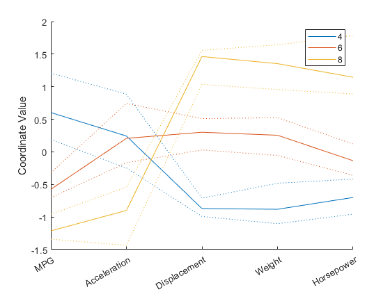
平行座標プロット
散布図行列では二変量の関係しか表示されませんが、すべての変数を一緒に表示して変数間の高次元の関係を調べることができるプロットもいくつかあります。最も簡単な多変量プロットは平行座標プロットです。このプロットの座標軸は、一般的な直交座標グラフのように直交するのではなく、水平に並べられています。各観測値はプロット内で、一連の結合されたライン セグメントとして表されます。
X の 4 気筒、6 気筒、または 8 気筒のすべての自動車のプロットを作成し、色を使って観測値をグループ化します。
cyl468 = ismember(Cylinders,[4 6 8]);
parallelcoords(X(cyl468,:),Group=Cylinders(cyl468), ...
    Standardize="on",Labels=varNames)

このプロットにおける水平方向は座標軸を表し、垂直方向はデータを表しています。各観測値は 5 つの変数に対する測定値から成り、各測定値は、対応する線が各座標軸と交差する高さとして表されます。5 つの変数で範囲が大きく異なるため、このプロットの各変数は平均が 0 で分散が 1 になるように標準化されています。グラフの色分けにより、8 気筒車は MPG と加速度の値が低く、排気量、重量、および馬力の値が高い傾向にあることがわかります。
平行座標プロットは、観測値の数が多いと読み取りにくくなることがあります。この問題を軽減するために、各グループについて中央値と第 1 四分位数および第 3 四分位数 (25% および 75% の点) のみを表示する平行座標プロットを作成できます。このプロットではグループ間の区別がわかりやすくなりますが、グループの外れ値などに関心がある場合、それらの観測値は含まれないため確認できません。
parallelcoords(X(cyl468,:),Group=Cylinders(cyl468), ...
    Standardize="on",Labels=varNames,Quantile=0.25)
アンドリュース プロット
多変量の可視化のもう 1 つのタイプにアンドリュース プロットがあります。このプロットは、区間 [0,1] における平滑化関数として各観測値を表します。
andrewsplot(X(cyl468,:),Group=Cylinders(cyl468),Standardize="on")
各関数は、対応する観測値に係数が等しいフーリエ級数です。この例では、フーリエ級数は 5 つの項をもっています。つまり、1 つの定数、周期が 1 と 1/2 の 2 つの正弦項、および 2 つの類似した余弦項です。最初の 3 つの項は、各関数の形状に対する影響が最も顕著に現れます。つまり、最初の 3 つの変数のパターンを最も容易に認識できます。
プロットでは、t = 0 の時点においてグループ間に明白な相違があります。この相違は、最初の変数 MPG が 4 気筒、6 気筒、または 8 気筒の自動車を互いに区別する特徴量の 1 つであることを示しています。t = 1/3 の辺りにおけるグループ間の相違も目を引きます。この値をアンドリュース プロット関数の式に入力します。結果は、変数の線形結合を定義する係数の集合になります。この線形結合は、グループを互いに区別するのに役立ちます。
t1 = 1/3;
coeffs = [1/sqrt(2) sin(2*pi*t1) cos(2*pi*t1) sin(4*pi*t1) cos(4*pi*t1)]
coeffs = 1×5

    0.7071    0.8660   -0.5000   -0.8660   -0.5000
これらの係数は、4 気筒車は 8 気筒車に比べて MPG と加速度の値が高く、排気量、馬力、および特に馬力の値は低いことを示しています。これは平行座標プロットから得られる結論と一致しています。
グリフ プロット
グリフを使用して次元を表すことで多変量データを可視化することもできます。関数 glyphplot では、スターおよびチャーノフのフェースという 2 種類のグリフを使用できます。データ セットの最初の 9 種類の型式について、それらの自動車のスター プロットを作成します。スターの各スポークは 1 つの変数を表し、スポークの長さはその観測値の変数の値に比例します。
g = glyphplot(X(1:9,:),Glyph="star",VarLabels=varNames, ...
    ObsLabels=Model(1:9,:));
set(g(:,3),FontSize=8);

このプロットでは、Figure ウィンドウでデータ カーソルを使用してデータ値を対話的に調べることができます。たとえば、Ford Torino のスターの右端のポイントをクリックすると、この自動車の MPG 値が 17 であることが示されます。
グリフ プロットと多次元尺度構成法
任意の順序でグリッド上にスターをプロットすると、隣接するスターの外観がまったく異なる図が作成されることがあります。いずれのパターンも視覚的に認識できない可能性があります。パターンを認識しやすくするには、多次元尺度構成法 (MDS) をグリフ プロットと組み合わせます。
まず、1977 年のすべての自動車を選択し、zscore 関数を使用して、5 つの各変数を平均が 0 で分散が 1 になるように標準化します。次に、標準化された観測値間のユークリッド距離を非類似度の尺度として計算します。より複雑な用途では、これよりも単純でない非類似度の尺度を使用することを検討してください。
models77 = find((Model_Year==77));
dissimilarity = pdist(zscore(X(models77,:)));
最後に、mdscale を使用して、点間距離が元の高次元のデータ点間の非類似度に近似するような 2 次元の位置の集合を作成します。それらの位置を使用してグリフをプロットします。結果の 2 次元プロットで、距離によってデータが大まかに再現されます。
Y = mdscale(dissimilarity,2);
figure
glyphplot(X(models77,:),Glyph="star",Centers=Y, ...
    VarLabels=varNames,ObsLabels=Model(models77,:),Radius=0.5)
title("1977 Model Year")
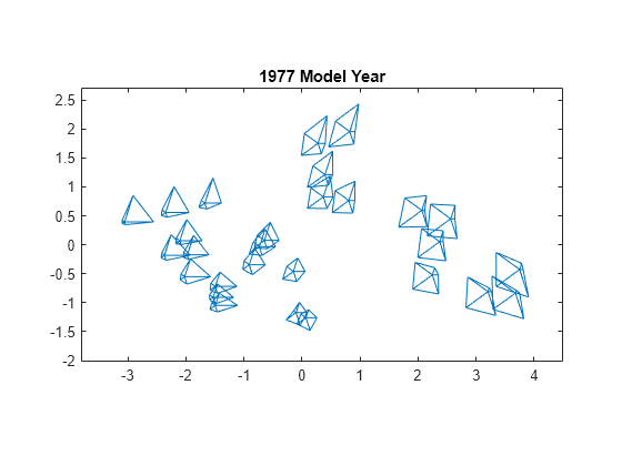
この 2 次元プロットでは、MDS を次元削減手法として使用しています。一般に、次元の削減は情報の損失を意味しますが、グリフによってすべての高次元情報がデータに組み込まれています。MDS を使用する目的は、データの変化に一定の規則性をもたせて、グリフ間のパターンをより簡単に認識できるようにすることです。
前のプロットと同様に、このプロットは Figure ウィンドウを使用して対話的に調べることができます。
別のタイプのグリフは、チャーノフのフェースです。このグリフは、各観測のデータ値をフェースの特徴量 (フェースの大きさ、フェースの形、目の位置など) にエンコードします。特徴量と変数との対応により、どの関係がプロットで最も認識しやすいかが決まります。この対応は glyphplot を使用して指定します。
figure
facePlot = glyphplot(X(models77,:),Glyph="face",Centers=Y, ...
    VarLabels=varNames,ObsLabels=Model(models77,:));
set(facePlot(:,1:2),Color="#D95319")
title("1977 Model Year")

このプロットでは、最もわかりやすい 2 つの特徴量 (フェースの大きさと額から顎までの相対的な大きさ) で MPG と加速度の変数をそれぞれエンコードしています。額と顎の形で排気量と重量の変数をそれぞれエンコードしています。目の間の幅で馬力の変数をエンコードしています。額が広くて顎が狭いフェースや額が狭くて顎が広いフェースが少ないことに注目してください。これは、排気量と重量の間に正の線形相関があることを示しています。この結果は散布図行列の結果と一致しています。
参考
gplotmatrix | parallelcoords | andrewsplot | glyphplot