判別分析分類器の正則化

この例では、モデルの予測力を損なわずに予測子の削除を試行して、よりロバストで簡潔なモデルを作成する方法を示します。これは、データに多数の予測子が含まれる場合に特に重要です。線形判別分析では、2 つの正則化パラメーター (ガンマとデルタ) を使用して冗長な予測子を特定および削除します。cvshrink メソッドはこれらのパラメーターの適切な設定の識別に役立ちます。

データを読み込み、分類器を作成する。

データ ovariancancer の線形判別分析分類器を作成します。結果のモデルを適度に小さく維持するために SaveMemory と FillCoeffs 名前と値のペアの引数を設定します。計算を容易にするため、この例では予測子の約 1/3 が含まれている無作為なサブセットを使用して分類器に学習させています。

load ovariancancer
rng(1); % For reproducibility
numPred = size(obs,2);
obs = obs(:,randsample(numPred,ceil(numPred/3)));
Mdl = fitcdiscr(obs,grp,'SaveMemory','on','FillCoeffs','off');

分類器の交差検証を実行する。

Gamma の 25 レベルと Delta の 25 レベルを使用して、適切なパラメーターを検索します。この検索には時間がかかります。進行状況を表示するために Verbose を 1 に設定します。

[err,gamma,delta,numpred] = cvshrink(Mdl,...
    'NumGamma',24,'NumDelta',24,'Verbose',1);

Done building cross-validated model.
Processing Gamma step 1 out of 25.
Processing Gamma step 2 out of 25.
Processing Gamma step 3 out of 25.
Processing Gamma step 4 out of 25.
Processing Gamma step 5 out of 25.
Processing Gamma step 6 out of 25.
Processing Gamma step 7 out of 25.
Processing Gamma step 8 out of 25.
Processing Gamma step 9 out of 25.
Processing Gamma step 10 out of 25.
Processing Gamma step 11 out of 25.
Processing Gamma step 12 out of 25.
Processing Gamma step 13 out of 25.
Processing Gamma step 14 out of 25.
Processing Gamma step 15 out of 25.
Processing Gamma step 16 out of 25.
Processing Gamma step 17 out of 25.
Processing Gamma step 18 out of 25.
Processing Gamma step 19 out of 25.
Processing Gamma step 20 out of 25.
Processing Gamma step 21 out of 25.
Processing Gamma step 22 out of 25.
Processing Gamma step 23 out of 25.
Processing Gamma step 24 out of 25.
Processing Gamma step 25 out of 25.

正則化分類器の品質を調べる。

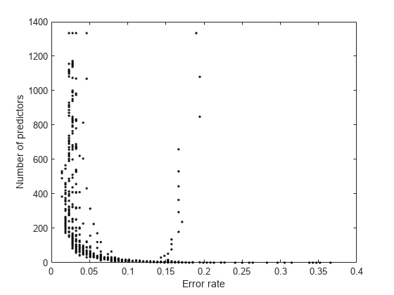
誤差に対する予測子の数をプロットします。

plot(err,numpred,'k.')
xlabel('Error rate')
ylabel('Number of predictors')

プロットの左下の部分をより詳しく調べます。

axis([0 .1 0 1000])

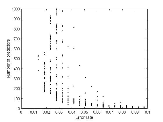
予測子の数が少ないことと誤差が少ないことは明らかにトレードオフの関係にあります。

モデルのサイズと精度の間の最適なトレードオフを選択する。

Gamma および Delta の値のペアには、ほぼ同じ最小誤差になるものが複数あります。このようなペアのインデックスと値を表示します。

まず、最小誤差値を見つけます。

minerr = min(min(err))

minerr = 0.0139

最小誤差を生成する err の添字を見つけます。

[p,q] = find(err < minerr + 1e-4);

添字から線形インデックスに変換します。

idx = sub2ind(size(delta),p,q);

Gamma と Delta の値を表示します。

[gamma(p) delta(idx)]

ans = 4×2

    0.7202    0.1145
    0.7602    0.1131
    0.8001    0.1128
    0.8001    0.1410

このような点は、非ゼロの係数がモデルに含まれている予測子全体の 29% しかありません。

numpred(idx)/ceil(numPred/3)*100

ans = 4×1

   39.8051
   38.9805
   36.8066
   28.7856

予測子の数をさらに減らすには、より大きな誤差率を受け入れなければなりません。たとえば、予測子の数が 200 以下で誤差率が最小となる Gamma および Delta を選択するには、次のようにします。

low200 = min(min(err(numpred <= 200)));
lownum = min(min(numpred(err == low200)));
[low200 lownum]

ans = 1×2

    0.0185  173.0000

0.0185 の誤差率を得るには、173 の予測子が必要ですが、これは 200 以下の予測子をもつ誤差率の中で最小です。

この誤差/予測子数になる Gamma と Delta を表示します。

[r,s] = find((err == low200) & (numpred == lownum));
[gamma(r); delta(r,s)]

ans = 2×1

    0.6403
    0.2399

正則化パラメーターを設定する。

Gamma および Delta のこれらの値をもつ分類器を設定するには、ドット表記を使用します。

Mdl.Gamma = gamma(r);
Mdl.Delta = delta(r,s);

ヒートマップのプロット

cvshrink の計算を Guo、Hastie および Tibshirani の計算[1]と比較するには、Gamma と Delta パラメーターのインデックスに対して、誤り率と予測子の数のヒートマップをプロットします (パラメーター Delta の範囲はパラメーター Gamma の値によって異なります。長方形のプロットを描画するには、パラメーター自体ではなくインデックス Delta を使用します)。

% Create the Delta index matrix
indx = repmat(1:size(delta,2),size(delta,1),1);

figure
subplot(1,2,1)
imagesc(err)
colorbar
colormap('jet')
title('Classification error')
xlabel('Delta index')
ylabel('Gamma index')

subplot(1,2,2)
imagesc(numpred)
colorbar
title('Number of predictors in the model')
xlabel('Delta index')
ylabel('Gamma index')

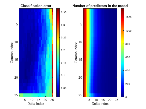
分類誤差は Delta が小さい場合に最適になりますが、予測子の数は Delta が大きいときが最も少なくなります。

参照

[1] Guo, Y., T. Hastie, and R. Tibshirani. "Regularized Discriminant Analysis and Its Application in Microarray." Biostatistics, Vol. 8, No. 1, pp. 86–100, 2007.

参考

関数

• fitcdiscr | cvshrink

オブジェクト

• ClassificationDiscriminant

関連するトピック

• 判別分析による分類
• 判別分析モデルの改善
• 特徴選択の紹介
• 機械学習モデルの解釈