Constraints in Bayesian Optimization
Bounds
bayesopt requires finite
bounds on all variables. (categorical variables
are, by nature, bounded in their possible values.) Pass the lower
and upper bounds for real and integer-valued variables in optimizableVariable.
bayesopt uses these bounds to sample points,
either uniformly or log-scaled. You set the scaling for sampling in optimizableVariable.
For example, to constrain a variable X1 to
values between 1e-6 and 1e3,
scaled logarithmically,
xvar = optimizableVariable('X1',[1e-6,1e3],'Transform','log')
bayesopt includes the endpoints in its range. Therefore, you cannot use 0
as a lower bound for a real log-transformed variable.
Tip
To use a zero lower bound in a real log-transformed variable, set the lower bound to
1, then inside the objective function use
x-1.
For an integer-valued log-transformed variable, you can use 0 as a lower bound. If
a lower bound is 0 for an integer-valued variable, then the software creates the
log-scaled space by using the log1p function instead of the
log function to include 0 in the variable sampling range.
log1p is a function that returns
log(1+x) for an input x.
Deterministic Constraints — XConstraintFcn
Sometimes your problem is valid or well-defined only for points
in a certain region, called the feasible region.
A deterministic constraint is a deterministic function that returns true when
a point is feasible, and false when a point is
infeasible. So deterministic constraints are not stochastic, and they
are not functions of a group of points, but of individual points.
Tip
It is more efficient to use optimizableVariable bounds,
instead of deterministic constraints, to confine the optimization
to a rectangular region.
Write a deterministic constraint function using the signature
tf = xconstraint(X)
Xis a width-D table of arbitrary height.tfis a logical column vector, wheretf(i) = trueexactly whenX(i,:)is feasible.
Pass the deterministic constraint function in the bayesopt
XConstraintFcn name-value argument. For example,
results = bayesopt(fun,vars,'XConstraintFcn',@xconstraint)
bayesopt evaluates deterministic
constraints on thousands of points, and so runs faster when your constraint
function is vectorized. See Vectorization.
For example, suppose that the variables named 'x1' and 'x2' are
feasible when the norm of the vector [x1 x2] is
less than 6, and when x1 <= x2.
The following constraint function evaluates these constraints.
function tf = xconstraint(X)
tf1 = sqrt(X.x1.^2 + X.x2.^2) < 6;
tf2 = X.x1 <= X.x2;
tf = tf1 & tf2;
Conditional Constraints — ConditionalVariableFcn
Conditional constraints are functions that enforce one of the following two conditions:
When some variables have certain values, other variables are set to given values.
When some variables have certain values, other variables have
NaNor, for categorical variables,<undefined>values.
Specify a conditional constraint by setting the bayesopt
ConditionalVariableFcn name-value argument to a function handle,
say @condvariablefcn. The @condvariablefcn
function must have the signature
Xnew = condvariablefcn(X)
Xis a width-Dtable of arbitrary height.Xnewis a table the same type and size asX.
condvariablefcn sets Xnew to
be equal to X, except it also sets the relevant
variables in each row of Xnew to the correct values
for the constraint.
Note
If you have both conditional constraints and deterministic constraints, bayesopt applies
the conditional constraints first. Therefore, if your conditional
constraint function can set variables to NaN or <undefined>,
ensure that your deterministic constraint function can process these
values correctly.
Conditional constraints ensure that variable values are sensible.
Therefore, bayesopt applies conditional constraints
first so that all passed values are sensible.
Conditional Constraint That Sets a Variable Value
Suppose that you are optimizing a classification using
fitcdiscr, and you optimize over both the
'DiscrimType' and 'Gamma' name-value
arguments. When 'DiscrimType' is one of the quadratic types,
'Gamma' must be 0 or the solver
errors. In that case, use this conditional constraint function:
function XTable = fitcdiscrCVF(XTable)
% Gamma must be 0 if discrim type is a quadratic
XTable.Gamma(ismember(XTable.DiscrimType, {'quadratic',...
        'diagQuadratic','pseudoQuadratic'})) = 0;
end
Conditional Constraint That Sets a Variable to NaN
Suppose that you are optimizing a classification using
fitcsvm, and you optimize over both the
'KernelFunction' and 'PolynomialOrder'
name-value arguments. When 'KernelFunction' is not
'polynomial', the 'PolynomialOrder'
setting does not apply. The following function enforces this conditional
constraint.
function Xnew = condvariablefcn(X)
Xnew = X;
Xnew.PolynomialOrder(Xnew.KernelFunction ~= 'polynomial') = NaN;
You can save a line of code as follows:
function X = condvariablefcn(X)
X.PolynomialOrder(X.KernelFunction ~= 'polynomial') = NaN;
In addition, define an objective function that does not pass the
'PolynomialOrder' name-value argument to
fitcsvm when the value of
'PolynomialOrder' is NaN.
fun = @(X)mysvmfun(X,predictors,responce,c)

function objective = mysvmfun(X,predictors,response,c)
    args = {predictors,response, ...
        'CVPartition',c, ...
        'KernelFunction',X.KernelFunction};
    if ~isnan(X.PolynomialOrder)
        args = [args,{'PolynomialOrder',X.PolynomialOrder}];
    end
    objective = kfoldLoss(fitcsvm(args{:}));
end
Coupled Constraints
Coupled constraints are constraints that you can evaluate only by calling the objective function. These constraints can be stochastic or deterministic. Return these constraint values from your objective function in the second argument. See Bayesian Optimization Objective Functions.
The objective function returns a numeric vector for the coupled constraints, one entry for each coupled constraint. For each entry, a negative value indicates that the constraint is satisfied (also called feasible). A positive value indicates that the constraint is not satisfied (infeasible).
bayesopt automatically creates a coupled
constraint, called the Error constraint, for every run. This constraint
enables bayesopt to model points that cause errors
in objective function evaluation. For details, see Objective Function Errors and predictError.
If you have coupled constraints in addition to the Error constraint:
Include the
NumCoupledConstraintsname-value argument in yourbayesoptcall (required). Do not include the Error constraint in this number.If any of your coupled constraints are stochastic, include the
AreCoupledConstraintsDeterministicname-value argument and passfalsefor any stochastic constraint.
Observe the coupled constraint values in each iteration by setting the
bayesopt
Verbose name-value argument to 1 or
2.
Note
When there are coupled constraints, iterative display and plot functions can give counterintuitive results such as:
A minimum objective plot can increase.
The optimization can declare a problem infeasible even when it showed an earlier feasible point.
The reason for this behavior is that the decision about whether
a point is feasible can change as the optimization progresses. bayesopt determines
feasibility with respect to its constraint model, and this model changes
as bayesopt evaluates points. So a “minimum
objective” plot can increase when the minimal point is later
deemed infeasible, and the iterative display can show a feasible point
that is later deemed infeasible.
For an example, see Bayesian Optimization with Coupled Constraints.
Bayesian Optimization with Coupled Constraints
A coupled constraint is one that can be evaluated only by evaluating the objective function. In this case, the objective function is the cross-validated loss of an SVM model. The coupled constraint is that the number of support vectors is no more than 100. The model details are in Optimize Cross-Validated Classifier Using bayesopt.
Create the data for classification.
rng default
grnpop = mvnrnd([1,0],eye(2),10);
redpop = mvnrnd([0,1],eye(2),10);
redpts = zeros(100,2);
grnpts = redpts;
for i = 1:100
    grnpts(i,:) = mvnrnd(grnpop(randi(10),:),eye(2)*0.02);
    redpts(i,:) = mvnrnd(redpop(randi(10),:),eye(2)*0.02);
end
cdata = [grnpts;redpts];
grp = ones(200,1);
grp(101:200) = -1;
c = cvpartition(200,'KFold',10);
sigma = optimizableVariable('sigma',[1e-5,1e5],'Transform','log');
box = optimizableVariable('box',[1e-5,1e5],'Transform','log');
The objective function is the cross-validation loss of the SVM model for partition c. The coupled constraint is the number of support vectors minus 100.5. This ensures that 100 support vectors give a negative constraint value, but 101 support vectors give a positive value. The model has 200 data points, so the coupled constraint values range from -99.5 (there is always at least one support vector) to 99.5. Positive values mean the constraint is not satisfied.
function [objective,constraint] = mysvmfun(x,cdata,grp,c)
SVMModel = fitcsvm(cdata,grp,'KernelFunction','rbf',...
    'BoxConstraint',x.box,...
    'KernelScale',x.sigma);
cvModel = crossval(SVMModel,'CVPartition',c);
objective = kfoldLoss(cvModel);
constraint = sum(SVMModel.IsSupportVector)-100.5;
Pass the partition c and fitting data cdata and grp to the objective function fun by creating fun as an anonymous function that incorporates this data. See Parameterizing Functions.
fun = @(x)mysvmfun(x,cdata,grp,c);
Set the NumCoupledConstraints to 1 so the optimizer knows that there is a coupled constraint. Set options to plot the constraint model.
results = bayesopt(fun,[sigma,box],'IsObjectiveDeterministic',true,...
    'NumCoupledConstraints',1,'PlotFcn',...
    {@plotMinObjective,@plotConstraintModels},...
    'AcquisitionFunctionName','expected-improvement-plus','Verbose',0);
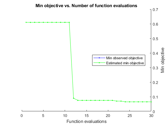
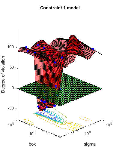
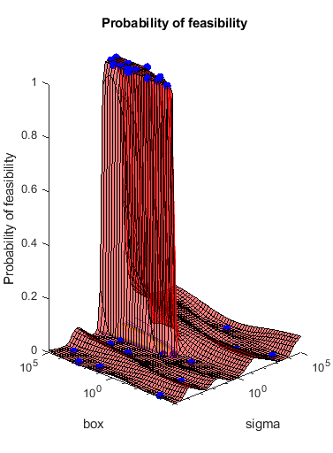
Most points lead to an infeasible number of support vectors.
See Also
bayesopt | optimizableVariable