Model Based Iterative Learning Control of Multi-Input Multi-Output System
This example shows how to implement model-based iterative learning control (ILC) to improve closed-loop trajectory tracking performance of a multi-input multi-output (MIMO) spring-mass-damper system. In this example, you design an ILC controller to perform a trajectory tracking for a second order MIMO plant, compare the model-based ILC results to a baseline PID controller, and show that an ILC controller provides a better tracking performance when augmented to a baseline controller.
Overview
ILC is an improvement in run-to-run control. It uses frequent measurements in the form of the error trajectory from the previous batch to update the control signal for the subsequent batch run. The focus of ILC is on improving the performance of systems that execute a single, repeated operation, starting at the same initial operating condition. This focus includes many practical industrial systems in manufacturing, robotics, and chemical processing, where mass production on an assembly line entails repetition. Therefore, use ILC when you have a repetitive task or repetitive disturbances and want to use knowledge from previous iteration to improve next iteration.
In general, ILC has two variations: model free and model based. Model-free ILC requires minimum information of your plant, which makes it easier to design and implement. Model-based ILC takes advantage of the additional knowledge of the plant, which can lead to faster convergence and better performance. In this example, you augment a baseline controller with a model-based ILC for reference tracking for a coupled mass-spring-damper system.
Mass-Spring-Damper System
The system consists of two carts of mass and , connected to each other and ground through springs with stiffness coefficient and , and dampers with damping coefficient .
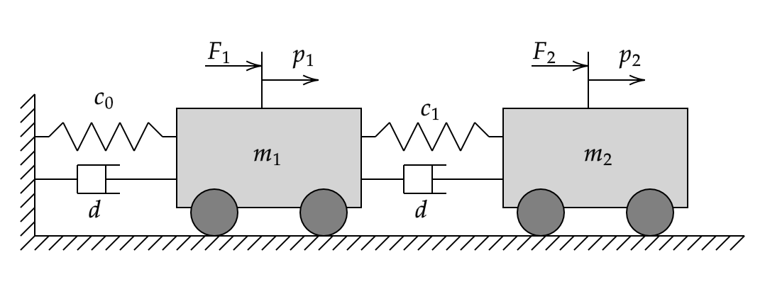
The state-space model defining the spring-mass-damper system can be written as follows:
.
Here, is the system states.
Specify the system parameters.
c0 = 1;
c1 = 1;
d = 1;
m1 = 1;
m2 = 1;
Define the mass-spring-damper state-space matrices.
A = [0 1 0 0;-(c0+c1)/m1 -2*d/m1 c1/m1 d/m1;...
     0 0 0 1; c1/m2 d/m2 -c1/m2 -2*d/m2];
B = [0 0;1/m1 0;...
     0 0;0 1/m2];
C = [1 0 0 0;...
     0 0 1 0];
D = zeros(2);
Define the sample time and iteration duration for ILC.
Ts = 0.01;
Tspan = 8;
Create a discrete-time state-space model with sample time Ts.
sysc = ss(A,B,C,D);
sys = c2d(sysc,Ts);
Examine Model
This examples provides a preconfigured Simulink® model. Open the model.
mdl = "scdModelBasedILCMIMO";
open_system(mdl)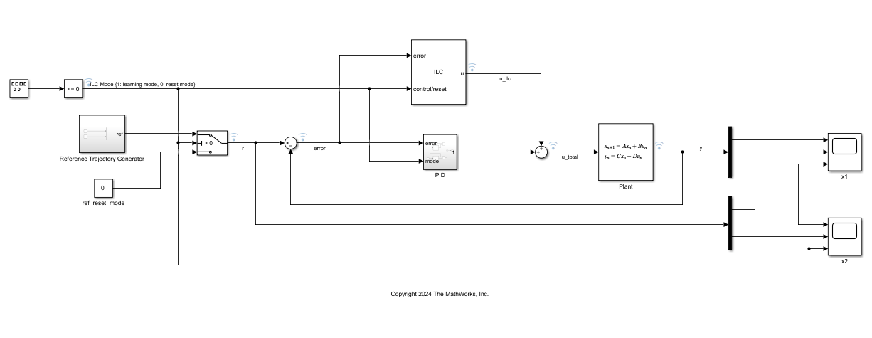
Baseline PID Controller
In this example, you use a switched PID controller as nominal control. For reference tracking (baseline control), the model uses a sluggish yet more robust baseline controller. To return the plant to its initial condition (reset), the model uses a more aggressive controller with larger transients.
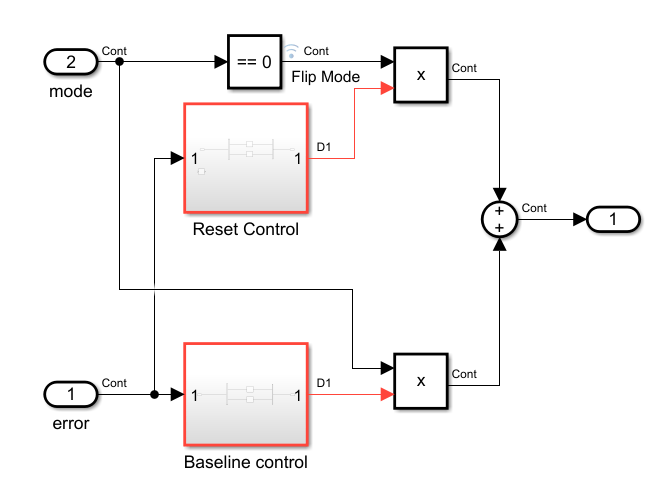
ILC Mode and Reference Generator
The ILC learning process involves two modes: learning and reset. In the learning mode, ILC outputs at the desired time points and measures the error between reference and output. At the end of the learning mode, ILC calculates the new control sequence to use in the next iteration. In the reset mode, the plant goes back to the initial operation condition, driven by the existing control mechanism. ILC output is 0 in the reset mode. The ILC Mode Generator subsystem defines the length of each mode and provides a signal that switches between the learning and reset modes.
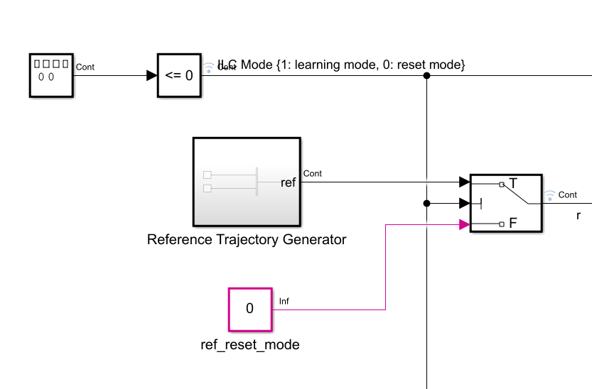
In this example, you use a generic sinusoidal reference signal for illustration purposes. In the learning mode, the reference signal is generated using the Reference Trajectory Generator subsystem. In the reset mode, the reference signal is zero, which allows the baseline PID controller to bring the plant back to the initial operating point.
Model-based ILC Controller
A model-based ILC controller uses the knowledge of the system dynamics and error feedback to update the control history for next iteration.
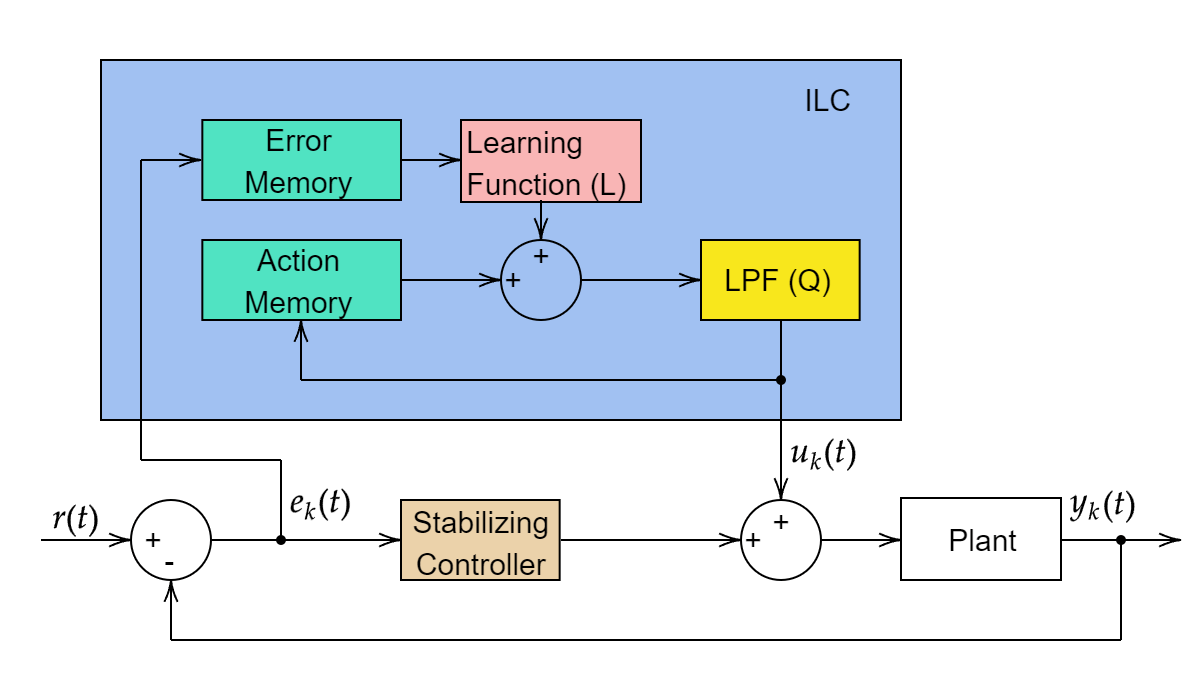
The controller update for model based-ILC ([1]) is defined by . Here:
is a low pass filter to filter out control chatter in the control
is learning rate.
is control history from iteration
is the error history from iteration
is the model-based update operator
Additionally, the iterative learning control block provides two types of model-based ILC: gradient based and inverse-model based [2].
Model-inversion based ILC uses the learning function .
Gradient-based ILC uses the learning function .
ILC Design
Define the control parameters for the model-based ILC for this MIMO tracking problem.
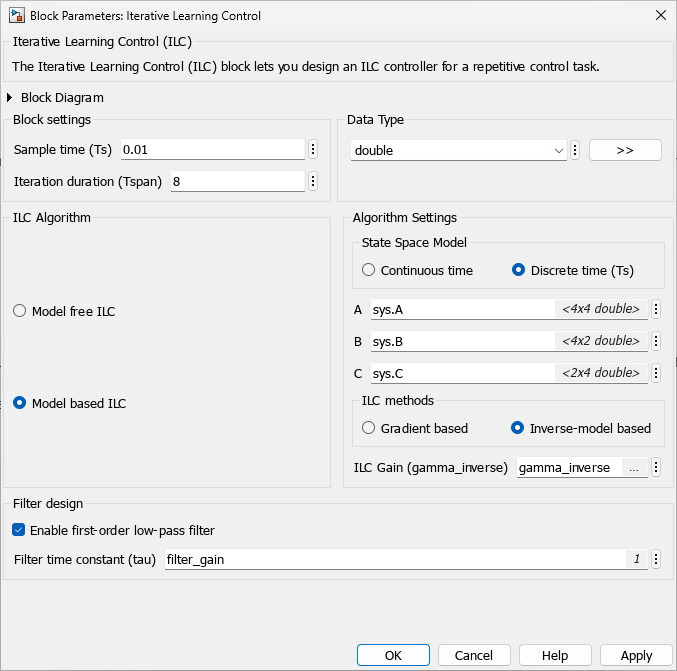
Set the learning rate for the model-inverse ILC control update.
gamma_inverse = 1.5;
The ILC controller uses a low pass filter to filter out any control chatter due to high learning rate. You can use the filter in ILC block by setting the filter time constant. Note that, for effective noise filtering, the filter time constant must be greater than or equal to the sample time Ts.
filter_gain = 1;
Simulate Model and Plot Results
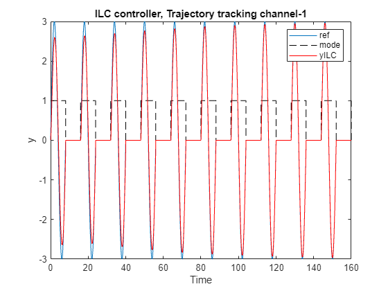
Simulate for 10 iterations (20*Tspan = 160 seconds). In the first iteration, ILC controller outputs 0 in the control mode because it just starts learning. Therefore, the closed-loop control performance displayed in the first iteration comes from the nominal controller, which serves as the baseline for the comparison.
simout_ilc = sim(mdl);
As the iterations progress, the ILC controller improves the reference tacking performance.
% Reference signal
r = squeeze(simout_ilc.logsout{8}.Values.Data);
% System output y_k
y_ilc = squeeze(simout_ilc.logsout{5}.Values.Data);
% Mode
mode = squeeze(simout_ilc.logsout{1}.Values.Data);
% plot output 'y' only for controlled part
y_ilc = y_ilc.*mode';
% Plots
figure(1)
plot(simout_ilc.logsout{8}.Values.Time, r(:,1))
hold on
plot(simout_ilc.logsout{1}.Values.Time, mode,'--','color','k')
plot(simout_ilc.logsout{3}.Values.Time, y_ilc(1,:),'color','r')
xlabel("Time")
ylabel("y")
legend("ref","mode","yILC")
title("ILC controller, Trajectory tracking channel-1")
hold off
figure(2)
plot(simout_ilc.logsout{4}.Values.Time, r(:,2))
hold on
plot(simout_ilc.logsout{1}.Values.Time, mode,'--','color','k')
plot(simout_ilc.logsout{3}.Values.Time, y_ilc(2,:),'color','r')
xlabel("Time")
ylabel("y")
legend("ref","mode","yILC")
title("ILC controller, Trajectory tracking channel-2")
hold off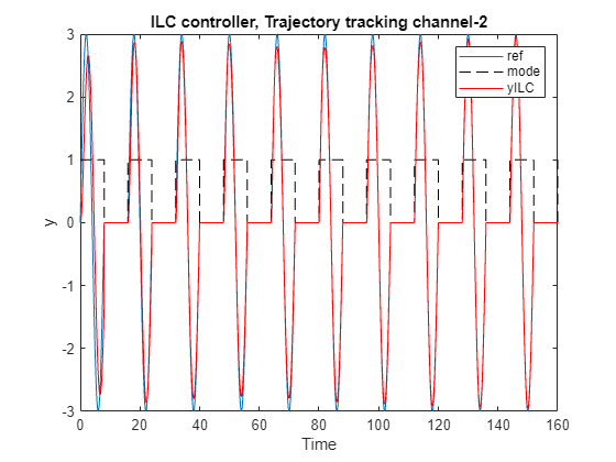
Plot the control effort of the ILC and PI controllers.
uILC = squeeze(simout_ilc.logsout{2}.Values.Data);
uILC = uILC.*mode';
uPID = squeeze(simout_ilc.logsout{4}.Values.Data);
tSim = simout_ilc.logsout{3}.Values.Time;
f = tiledlayout(2,2,TileSpacing="tight");
%Plot ILC control for channel-1
nexttile
plot(tSim,uILC(1,:))
xlabel("Time")
ylabel("u");
title("ILC Control Channel-1")

%Plot PID control for channel-1
nexttile
plot(tSim,uPID(:,1),'color','r')
xlabel("Time")
ylabel("u");
title("PID Control Channel-1")

%Plot ILC control for channel-2
nexttile
plot(tSim,uILC(2,:))
xlabel("Time")
ylabel("u");
title("ILC Control Channel-2")

%Plot PID control for channel-2
nexttile
plot(tSim,uPID(:,2),'color','r')
xlabel("Time")
ylabel("u");
title("PID Control Channel-2")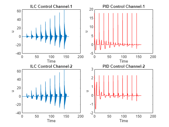
As iterations progress the ILC controller learns to compensate for the tracking error and the nominal PID control effort is reduced to a minimum.
References
Bristow, Douglas A., Marina Tharayil, and Andrew G. Alleyne. “A Survey of Iterative Learning Control.” IEEE Control Systems 26, no. 3 (June 2006): 96–114.
Zhang, Yueqing, Bing Chu, and Zhan Shu. “A Preliminary Study on the Relationship Between Iterative Learning Control and Reinforcement Learning⁎.” IFAC-PapersOnLine, 13th IFAC Workshop on Adaptive and Learning Control Systems ALCOS 2019, 52, no. 29 (January 1, 2019): 314–19.