モデルの参照時にローカル ソルバーを使用
モデル コンフィギュレーション ペイン: モデル参照
説明
[モデルの参照時にローカル ソルバーを使用] コンフィギュレーション パラメーターは、参照モデルによって実装されるシステムを解く方法を指定します。このパラメーターを選択すると、現在の参照モデルの [ソルバー] コンフィギュレーション パラメーターに指定されているソルバーを使用して、参照モデルが一連の別個の微分方程式セットとして解かれます。
固定ステップ ローカル ソルバーの場合、参照モデルの [固定ステップ サイズ (基本サンプル時間)] コンフィギュレーション パラメーターを使用して、ローカル ソルバーの固定ステップ サイズを指定します。
可変ステップ ローカル ソルバー (R2025a 以降)の場合、参照モデルの [最大ステップ サイズ]、[最小ステップ サイズ]、[初期ステップ サイズ]、[相対許容誤差]、[絶対許容誤差] の各コンフィギュレーション パラメーターを使用して、ローカル ソルバーの可変ステップ サイズを決定する基準を指定します。
ローカル ソルバーを使用することで、システムの構成と統合を促進できます。ローカル ソルバーを使用すると、各モデルを別個に設計およびテストするのに使用したのと同じソルバーとステップ サイズを使用して、システムレベルのシミュレーションで参照モデルを解くことができます。また、ローカル ソルバーを使用すれば、モデルをより大規模なシステムに統合しながら、参照モデルのコンフィギュレーション パラメーターに必要なコンフィギュレーションの調整量を減らすこともできます。
一部のシステムでは、ローカル ソルバーを使用すると、参照モデル内のシステムを解くのにより適切なソルバーを選択できるようになったり、複数のコンポーネントに幅広いダイナミクスがあるシステムでの冗長な計算の数を減らしたりできるため、シミュレーションのパフォーマンスを向上させることができます。
例については、Improve Simulation Performance by Using Local Solversを参照してください。
ローカル ソルバーの詳細については、Use Local Solvers in Referenced Modelsを参照してください。
参照モデルのコンフィギュレーション パラメーターの設定
モデル参照階層では、最上位モデルと現在の参照モデルのどちらのパラメーターを編集するかは、[コンフィギュレーション パラメーター] ダイアログ ボックスへのアクセス方法によって変わります。
現在のモデルの階層構造における最上位モデル — Simulink® ツールストリップの [モデル化] タブで [モデル設定] をクリックします。
現在の参照モデル — Simulink ツールストリップの [モデル化] タブで [モデル設定] ボタンの矢印をクリックします。その後、[参照モデル] セクションで [モデル設定] を選択します。
あるいは、参照モデルを最上位モデルとして開きます。その後、Simulink ツールストリップの [モデル化] タブで [モデル設定] をクリックします。
設定
off (既定値) | ononローカル ソルバーを使用して参照モデルを一連の別個の微分方程式として解きます。ローカル ソルバーは、参照モデルの [ソルバー] コンフィギュレーション パラメーターを使用して指定します。
off親ソルバーを使用して参照モデルを親システムの一部として解かれます。
例
モデル SecondOrderSystemTop を開きます。このモデルには、2 次システムのモデルを参照する Model ブロックに入力信号を提供する Ramp ブロックが含まれています。Model ブロックの出力信号は Outport ブロックに接続されます。
topmdl = "SecondOrderSystemTop";
open_system(topmdl)
参照モデル内を移動するには、Model ブロックをダブルクリックします。あるいは、Model ブロックの Simulink.BlockPath オブジェクトを作成し、関数 open を使用してモデルの階層構造のコンテキストで参照モデルを開きます。
mdlblkpath = Simulink.BlockPath(topmdl + "/Model");
open(mdlblkpath)
参照モデルは、Transfer Fcn ブロックを使用して 2 次システムを実装し、システムへの変更または外乱をモデル化する Step ブロックを含みます。
システム伝達関数は、2 つのモデル ワークスペース変数 wn と z を使用して Transfer Fcn ブロックで指定します。これらの変数はシステムの固有振動数 (ラジアン/秒) とシステムの減衰係数を表します。
モデル ワークスペースで変数 wn の値を 100 として指定して、固有振動数 100 ラジアン/秒でシステムを構成します。
refmdl = "SecondOrderSystem";
mdlwksp = get_param(refmdl,"ModelWorkspace");
assignin(mdlwksp,"wn",100)
ステップ サイズ 0.01 秒でローカル ソルバーを使用するように参照モデルを構成します。プロパティ インスペクターまたは [ブロック パラメーター] ダイアログ ボックスを使用して、最上位モデルから参照モデルの設定を構成できます。
プロパティ インスペクターを開きます。[モデル化] タブで [設計] セクションを展開し、[プロパティ インスペクター] を選択するか、Ctrl+Shift+I を押します。
参照モデルの [コンフィギュレーション パラメーター] ダイアログ ボックスを開くには、Model ブロックを選択します。次に、プロパティ インスペクターで [ソルバー] セクションを展開し、[ローカル ソルバーを使用] パラメーターの横にあるハイパーリンクをクリックします。
モデルの階層構造内で参照されている場合にローカル ソルバーを使用するようにモデルを構成します。[コンフィギュレーション パラメーター] ダイアログ ボックスの [モデル参照] ペインで、[モデルの参照時にローカル ソルバーを使用] を選択します。
ローカル ソルバーとして固定ステップ
ode3を選択します。[ソルバー] ペインの [タイプ] リストから[Fixed-step]を選択します。次に、[ソルバー] リストから[ode3 (Bogacki-Shampine)]を選択します。ローカル ソルバーのステップ サイズを 0.01 秒に設定します。[ソルバー] ペインで、[ソルバーの詳細] を展開します。次に、[固定ステップ サイズ (基本サンプル時間)] ボックスに「
0.01」と入力します。[OK] をクリックします。
あるいは、関数 set_param を使用してパラメーターを構成します。
set_param(refmdl,UseModelRefSolver="on",...
    SolverType="Fixed-Step",Solver="ode3",FixedStep="0.01")
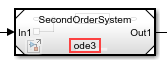
最上位モデルの Model ブロックに、指定したローカル ソルバーが示されます。

モデル参照の "通信ステップ サイズ" を指定します。通信ステップ サイズは、親ソルバーとローカル ソルバーがデータを交換するタイミングを指定し、最上位モデルの離散サンプル時間として登録されます。
最上位モデルの Ramp ブロックの傾きは 0.2 で、最上位ソルバーはステップ サイズ 0.2 秒を使用します。最上位モデルからの入力信号は 2 次システムのダイナミクスに比べてゆっくりと変化するため、シミュレーション結果の精度に大きな影響を与えることなく、通信ステップ サイズをローカル ソルバーのステップ サイズよりも大幅に大きくすることができます。
通信ステップ サイズを 0.4 秒に指定します。Model ブロックを選択します。次に、プロパティ インスペクターの [ソルバー] の下の [通信ステップ サイズ] ボックスに「0.4」と入力します。
あるいは、関数 set_param を使用して CommunicationStepSize パラメーターを設定します。
set_param(topmdl + "/Model",CommunicationStepSize="0.4")
ローカル ソルバーを使用してモデルをシミュレーションし、2 次システムの応答を計算します。
out = sim(topmdl);
シミュレーション結果を表示するには、シミュレーション データ インスペクターを開きます。[シミュレーション] タブの [結果の確認] で、[データ インスペクター] をクリックします。あるいは、関数 Simulink.sdi.view を呼び出します。
Simulink.sdi.view
別個のサブプロットに System Response および System Response - Top という名前の信号をプロットします。あるいは、関数 Simulink.sdi.loadView を使用して、この例で作成された FastSecondOrderSystem という名前のビューを読み込みます。
Simulink.sdi.loadView("FastSecondOrderSystem.mldatx");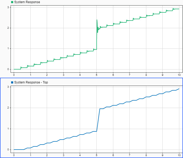
System Response 信号と System Response - Top 信号は同じ信号ですが、異なる場所にログが記録されます。System Response 信号は、ローカル ソルバーのステップ サイズによって決定されるレートで参照モデル内にログが記録されます。System Response - Top 信号は、最上位ソルバーのステップ サイズによって決定されるレートで、最上位モデルの Outport ブロックによってログが記録されます。ローカル ソルバーのステップ サイズは最上位ソルバーのステップ サイズよりもはるかに小さいため、System Response 信号は、Step ブロックの出力値が変化したときの入力信号の変化に対するシステム応答をより高い忠実度で取得します。
System Response 信号では、ローカル ソルバーが各通信ステップ間にゼロ次ホールドを使用して入力信号を内挿する効果がわかります。時間軸の 5 秒付近を拡大すると、ステップに対するシステム応答の振動がわかります。

モデル SecondOrderSystemTop を開きます。このモデルには、2 次システムのモデルを参照する Model ブロックに入力信号を提供する Ramp ブロックが含まれています。Model ブロックの出力信号は Outport ブロックに接続されます。
topmdl = "SecondOrderSystemTop";
open_system(topmdl)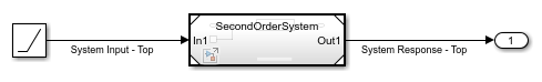
参照モデル内を移動するには、Model ブロックをダブルクリックします。あるいは、Model ブロックの Simulink.BlockPath オブジェクトを作成し、関数 open を使用してモデルの階層構造のコンテキストで参照モデルを開きます。
mdlblkpath = Simulink.BlockPath(topmdl + "/Model");
open(mdlblkpath)
参照モデルは、Transfer Fcn ブロックを使用して 2 次システムを実装し、システムへの変更または外乱をモデル化する Step ブロックを含みます。
システム伝達関数は、2 つのモデル ワークスペース変数 wn と z を使用して Transfer Fcn ブロックで指定します。これらの変数はシステムの固有振動数 (ラジアン/秒) とシステムの減衰係数を表します。
モデル ワークスペースで変数 wn の値を 1 として指定して、固有振動数 1 ラジアン/秒でシステムを構成します。
refmdl = "SecondOrderSystem";
mdlwksp = get_param(refmdl,"ModelWorkspace");
assignin(mdlwksp,"wn",1)
ステップ サイズ 0.4 秒でローカル ソルバーを使用するように参照モデルを構成します。プロパティ インスペクターまたは [ブロック パラメーター] ダイアログ ボックスを使用して、最上位モデルから参照モデルの設定を構成できます。
プロパティ インスペクターを開きます。[モデル化] タブで [設計] セクションを展開し、[プロパティ インスペクター] を選択するか、Ctrl+Shift+I を押します。
参照モデルの [コンフィギュレーション パラメーター] ダイアログ ボックスを開くには、Model ブロックを選択します。次に、プロパティ インスペクターで [ソルバー] セクションを展開し、[ローカル ソルバーを使用] パラメーターの横にあるハイパーリンクをクリックします。
モデルの階層構造内で参照されている場合にローカル ソルバーを使用するようにモデルを構成します。[コンフィギュレーション パラメーター] ダイアログ ボックスの [モデル参照] ペインで、[モデルの参照時にローカル ソルバーを使用] を選択します。
ローカル ソルバーとして固定ステップ
ode3を選択します。[ソルバー] ペインの [タイプ] リストから[Fixed-step]を選択します。次に、[ソルバー] リストから[ode3 (Bogacki-Shampine)]を選択します。ローカル ソルバーのステップ サイズを 0.4 秒に設定します。[ソルバー] ペインで、[ソルバーの詳細] を展開します。次に、[固定ステップ サイズ (基本サンプル時間)] ボックスに「
0.4」と入力します。[OK] をクリックします。
あるいは、関数 set_param を使用してパラメーターを構成します。
set_param(refmdl,UseModelRefSolver="on",...
    SolverType="Fixed-Step",Solver="ode3",FixedStep="0.4")
最上位モデルの Model ブロックに、指定したローカル ソルバーが示されます。
ローカル ソルバーのステップ サイズが親ソルバーのステップ サイズより大きい場合、[通信ステップ サイズ] パラメーターを -1 に指定することで、"通信ステップ サイズ" を継承します。通信ステップ サイズは、親ソルバーとローカル ソルバーがデータを交換するタイミングを指定し、親モデルの離散サンプル時間として登録されます。
set_param(topmdl + "/Model",CommunicationStepSize="-1")
ローカル ソルバーを使用してモデルをシミュレーションし、2 次システムの応答を計算します。
out = sim(topmdl,StopTime="20");シミュレーション結果を表示するには、シミュレーション データ インスペクターを開きます。[シミュレーション] タブの [結果の確認] で、[データ インスペクター] をクリックします。あるいは、関数 Simulink.sdi.view を呼び出します。
Simulink.sdi.view
別個のサブプロットに System Response および System Response - Top という名前の信号をプロットします。あるいは、関数 Simulink.sdi.loadView を使用して、この例で作成された SlowSecondOrderSystem という名前のビューを読み込みます。
Simulink.sdi.loadView("SlowSecondOrderSystem.mldatx");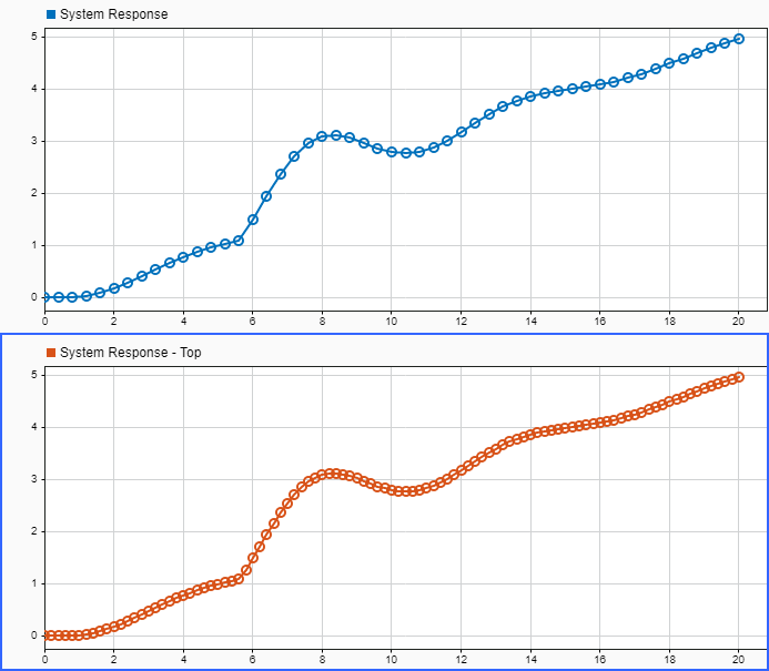
System Response 信号と System Response - Top 信号は同じ信号ですが、異なる場所にログが記録されます。System Response 信号は、ローカル ソルバーのステップ サイズによって決定されるレートで参照モデル内にログが記録されます。System Response - Top 信号は、最上位ソルバーのステップ サイズによって決定されるレートで、最上位モデルの Outport ブロックによってログが記録されます。ローカル ソルバーのステップ サイズが親ソルバーのステップ サイズよりも大きいため、System Response 信号についてログに記録されるデータ点の数が少なくなります。
ヒント
Model ブロックのパラメーターを使用して以下を指定できます。
ローカル ソルバーと親ソルバーの間でデータを交換するレートを指定する "通信ステップ サイズ"
親ソルバーからの入力をローカル ソルバーで外挿する方法
出力信号値を親ソルバーに提供するために状態や出力の値をローカル ソルバーで内挿する方法
R2024a より前: 最上位のソルバーが固定ステップ ソルバーの場合、ローカル ソルバーのステップ サイズは親ソルバーのステップ サイズの整数倍でなければなりません。
推奨設定
| アプリケーション | 設定 |
|---|---|
| デバッグ | off |
| トレーサビリティ | 影響なし |
| 効率性 | 推奨なし |
| 安全対策 | 影響なし |
プログラムでの使用
パラメーター: UseModelRefSolver |
値: "on" | "off" |
既定の設定: "off" |