Main Content

latency

Calculate propagation delay from one asset to another asset

Since R2023a

    Description

    delay = latency(source,target) calculates the history of propagation delays from the source asset to the target asset. The source and target assets must belong to the same satelliteScenario object. If the value of the AutoSimulate property of the satelliteScenario object is true, the latency function returns the propagation delay history from the value of StartTime to the value of StopTime. Otherwise, it returns the propagation delay history from StartTime to SimulationTime.

    [delay,timeOut] = latency(source,target) returns the history of time samples timeOut.

    [___] = latency(source,target,timeIn) calculates latency at the specified datetime timeIn. When using this syntax, the latency function sets the second dimension of delay and timeOut to 1.

    Note

    When the target asset is a Satellite object, the latency function uses a numerical iterative solution to compute the propagation delay. When the target asset is a GroundStation object, the latency function applies Sagnac correction to compute the propagation delay.

    Examples

    collapse all

    Determine the history of propagation delay from a satellite to a ground station. Also, determine the corresponding time samples.

    Create a satelliteScenario object.

    startTime = datetime(2022,8,21);                       % August 21, 2022, 12:00 AM UTC
    stopTime = datetime(2022,8,23);                        % August 23, 2022, 12:00 AM UTC
    sampleTime = 60;                                       % Units are in seconds
    sc = satelliteScenario(startTime,stopTime,sampleTime);

    Add a satellite to the scenario.

    semiMajorAxis = 10000000;             % In meters
    eccentricity = 0;
    inclination = 0;                      % In degrees
    rightAscensionOfAscendingNode = 0;    % In degrees
    argumentOfPeriapsis = 0;              % In degrees
    trueAnomaly = 0;                      % In degrees
    sat = satellite(sc,semiMajorAxis,eccentricity,inclination,rightAscensionOfAscendingNode,argumentOfPeriapsis,trueAnomaly);

    Add a ground station to the scenario.

    gs = groundStation(sc);

    Determine the propagation delay history between two assets and the corresponding time samples.

    [delay,timeOut] = latency(sat,gs);

    Input Arguments

    collapse all

    Source asset from scenario, specified as a Satellite object, Platform object, GroundStation object, array of Satellite objects, array of Platform objects, or array of GroundStation objects.

    Target asset from scenario, specified as a Satellite object, Platform object, GroundStation object, array of Satellite objects, array of Platform objects, or array of GroundStation objects.

    Time instance at which the function calculates latency, specified as a datetime scalar. If timeIn does not specify a time zone, the function uses Coordinated Universal Time (UTC).

    Data Types: datetime

    Output Arguments

    collapse all

    Delay, in seconds, returned as a scalar, vector, or matrix. When source and target cannot access each other, the corresponding latency value is NaN. These tables show how this output changes based on the different input argument sizes and combinations.

    • timeIn not specified

      sourcetargetdelayDescription
      scalarscalarrow vectorLatency history, in which each element represents the propagation delay from source to target at a specific time.
      scalarvectormatrixEach row represents the propagation delay from source to target. The row index indicates the position of the asset in target.
      vectorscalarmatrixEach row represents the propagation delay from source to target. The row index indicates the position of the asset in source.
      vectorvectormatrixEach row represents the propagation delay from source to target. The row index indicates the position of the assets in source and target.

    • timeIn specified

      sourcetargetdelayDescription
      scalarscalarscalarLatency at the specified datetime timeIn.
      scalarvectorcolumn vectorEach element represents the propagation delay from source to the corresponding asset in target at the specified datetime timeIn.
      vectorscalarcolumn vectorEach element represents the propagation delay from the corresponding asset in source to target at the specified datetime timeIn.
      vectorvectorcolumn vectorEach element represents the propagation delay between the corresponding pair of source and target assets at the specified datetime timeIn.

    Data Types: double

    Time samples between the start and stop time of the scenario, returned as a scalar or vector.

    If timeIn does not specify a time zone and the AutoSimulate property the satelliteScenario object is true, the latency function returns the time sample history from StartTime to StopTime. Otherwise, it returns the time sample history from the value of StartTime to the value of SimulationTime.

    Data Types: datetime

    More About

    collapse all

    Latency When Ground Station Is Target

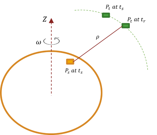
    Consider a satellite scenario in which a satellite is the source and a ground station on Earth is the target. Because the satellite scenario currently supports only static ground stations, assume that the velocity of the ground station is the same as the angular velocity of Earth.

    Given the instant at which the source transmits the signal ts and the instant at which the target receives the signal tr, the latency or propagation delay is the difference trts. Assume that at every instant, the source transmits the signal. The unknown is the instant at which the signal reaches the target.

    A diagrammatic view of a ground station as target

    Consider that the positions of the source and the target are in International Terrestrial Reference Frame (ITRF).

    • Source position Ps at ts[x y z]

    • Target position Pt at tr[a,b,d]

    The distance between the target position Pt and the source position Ps in the tr time frame is the distance travelled by the signal ρ, where ρ=PttrPstr.

    To obtain the source position in the tr time frame, apply this rotation matrix to the source position.

    Rtstr=[cos(ω(trts))sin(ω(trts))0sin(ω(trts))cos(ω(trts))0001]

    In this equation, the time difference trts equals the time taken by the signal to cover the distance ρ.

    trts=ρc.

    Substitute this value in the rotation matrix to obtain

    Rtstr=[cos(ωρc)sin(ωρc)0sin(ωρc)cos(ωρc)0001].

    The position of source in the time frame tr is

    Pstr=RtstrPsts.

    Pstr=[cos(ωρc)sin(ωρc)0sin(ωρc)cos(ωρc)0001][xyz].

    In this equation,

    • ω is to the order of 1e-5.

    • ρ is to the order of 1e7.

    • c is to the order of 1e-8.

    • ωρc is to the order of 1e-5.

    As ωρc is very small, apply small angle approximation (sin(θ)θ and cos(θ)1) to obtain

    Pstr=[1ωρc0ωρc10001][xyz].

    Substitute this value in ρ=PttrPstr to obtain

    ρ=((xa)+yωρc)2+(xωρc+(yb))2+(zd)2.

    Square both sides of this equation to obtain

    ρ2=((xa)2+(yωρc)2+2(xa)(yωρc))+((yb)2+(xωρc)22(yb)(xωρc))+(zd)2.

    Rearrange the terms and simplify the equation to obtain

    ρ2=(xa)2+(yb)2+(zd)2+((ωρc)2(x2+y2)+2ωρc(bxay)).

    The true geometric range for the position of source and target in the tr time frame is

    r2=((ax)2+(by)2+(dz)2).

    Let Rcorr=ωc(bxay) and e1=(ωc)2(x2+y2). Substitute these values in ρ2=(xa)2+(yb)2+(zd)2+((ωρc)2(x2+y2)+2ωρc(bxay)) to obtain

    ρ2=r2+(e1ρ2+2ρRcorr).

    (1e1)ρ22ρRcorrr2=0.

    The discriminant of this quadratic equation is

    discriminant=4Rcorr2+4(1e1)r2.

    ρ=2Rcorr+discriminant2(1e1).

    If Rcorrr(1e1), then you can express ρ as

    ρ=2Rcorr+2r1e12(1e1)=Rcorr(1e1)+r1e1.

    Latency When Satellite Is Target

    When the target is a satellite, you must consider the movement of a satellite to know when the satellite receives the signal.

    Let f be the function that defines the orbital motion of the satellite, which is nonlinear with no sharp peaks. Also, let PS be the position of the source in Geocentric Celestial Reference Frame (GCRF). The time taken by the signal to reach the target equals the time the target takes to move from its position at the transmission time to its position at the reception time.

    You can find the solution for the objective function iteratively by using the Newton-Raphson method.

    ObjectiveFunction(t)=(f(tS+t)PSc)t, where tS is the source transmit time.

    Assuming the satellite does not move, the initial guess to the function is the time the signal takes to reach the satellite.

    The root of the objective function is latency. Obtaining the exact root is not always possible because of the numerical precision errors. Therefore, consider the value for which the objective function returns a value less than 2.2204e-16 as the root.

    A diagrammatic view of a satellite as target

    This methodology is applicable for any moving target, regardless of source movement.

    Version History

    Introduced in R2023a