このページは機械翻訳を使用して翻訳されました。最新版の英語を参照するには、ここをクリックします。
衛星シナリオにおけるレイテンシとドップラー効果の計算
この例では、SEM アルマナックから GPS 衛星コンステレーションをモデル化し、衛星と地上局間のアクセスを解析し、衛星と地上局間の遅延とドップラーシフトを計算する方法を示します。
衛星シナリオを作成する
開始時刻が 2020 年 1 月 11 日PM2 時 50 分 UTC、終了時刻が 3 日後の衛星シナリオを作成します。シミュレーションのサンプル時間を 60 秒に設定します。
startTime = datetime(2020,1,11,14,50,0);
stopTime = startTime + days(3);
sampleTime = 60;                         % In seconds
sc = satelliteScenario( ...
    startTime,stopTime,sampleTime);
シナリオに衛星を追加する
gpsAlmanac.txt SEMアルマナックファイルからシナリオに衛星を追加します。最新の SEMアルマナックファイルを入手するには、ナビゲーション センターの Web サイト (www.navcen.uscg.gov) にアクセスし、「SEMアルマナック」を検索してください。
sat = satellite(sc,"gpsAlmanac.txt");SEMアルマナックを使用して衛星を作成する場合のデフォルトの軌道プロパゲーターは gps です。これは、OrbitPropagator プロパティを観察することで確認できます。さらに、orbitalElements 関数の出力にはGPS衛星固有の情報が含まれます。
orbitProp = sat(1).OrbitPropagator
orbitProp =
"gps"
elements = orbitalElements(sat(1))
elements = struct with fields:
                                  PRN: 1
                        GPSWeekNumber: 2087
               GPSTimeOfApplicability: 589824
                      SatelliteHealth: 0
                        SemiMajorAxis: 2.6560e+07
                         Eccentricity: 0.0093
                          Inclination: 56.0665
    GeographicLongitudeOfOrbitalPlane: -40.4778
                 RateOfRightAscension: -4.6166e-07
                    ArgumentOfPerigee: 43.3831
                          MeanAnomaly: 172.6437
                               Period: 4.3077e+04
地上局を追加する
マドリード深宇宙通信複合施設を対象の地上局として追加し、その緯度と経度を指定します。
name = "Madrid Deep Space Communications Complex";
lat = 40.43139;                                    % In degrees
lon = -4.24806;                                    % In degrees
gs = groundStation(sc, ...
    Name=name,Latitude=lat,Longitude=lon);
アクセス解析と可視化シナリオを追加する
GPS 衛星とマドリード地上局間のアクセス解析を追加します。これにより、地上局が衛星から見えるタイミングが決定されます。これは、時間の経過とともに地上局からどの衛星が見えるかを可視化するのに役立ちます。
ac = access(sat,gs);
衛星シナリオ ビューアーを起動してシナリオを可視化します。可視化が乱雑にならないように、ビューアの ShowDetails を false に設定します。地上局にアクセスできるすべての衛星が視界に入るようにカメラの位置を設定します。
v = satelliteScenarioViewer(sc,ShowDetails=false);
campos(v, ...
    29, ...                                        % Latitude in degrees
    -19, ...                                       % Longitude in degrees
    7.3e7);                                        % Altitude in meters

レイテンシとレイテンシの変化率を計算する
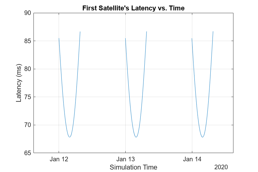
latency 関数を使用して、 GPS衛星からマドリード地上局までの伝播遅延を計算します。また、伝播遅延の変化率を計算します。
% Calculate propagation delay from each satellite to the ground station.
% The latency function internally performs access analysis and returns NaN
% whenever there is no access.
[delay,time] = latency(sat,gs);
最初の衛星に対応する伝播遅延をプロットします。すべての衛星に対応する伝播遅延をプロットすることもできます。ただし、この例では、デモンストレーションとして、またプロットの乱雑さを軽減するために、最初の衛星のみをプロットします。
plot(time,delay(1,:)*1000)                  % Plot in milliseconds
xlim([time(1) time(end)])
title("First Satellite's Latency vs. Time")
xlabel("Simulation Time")
ylabel("Latency (ms)")
grid on
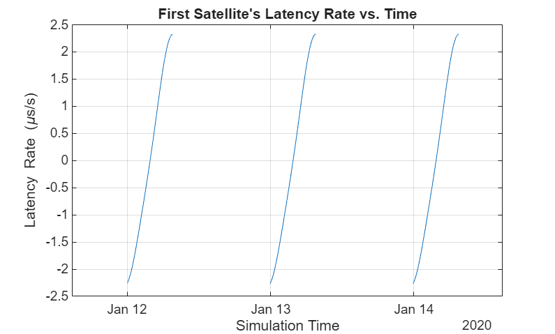
最初の衛星に対応する伝播遅延の変化率をプロットします。
latencyRate = diff(delay,1,2)/sampleTime;
plot(time(1:end-1),latencyRate(1,:)*1e6)          % Plot in microseconds/second
xlim([time(1) time(end-1)])
title("First Satellite's Latency Rate vs. Time")
xlabel("Simulation Time")
ylabel("Latency Rate (\mus/s)")
grid on
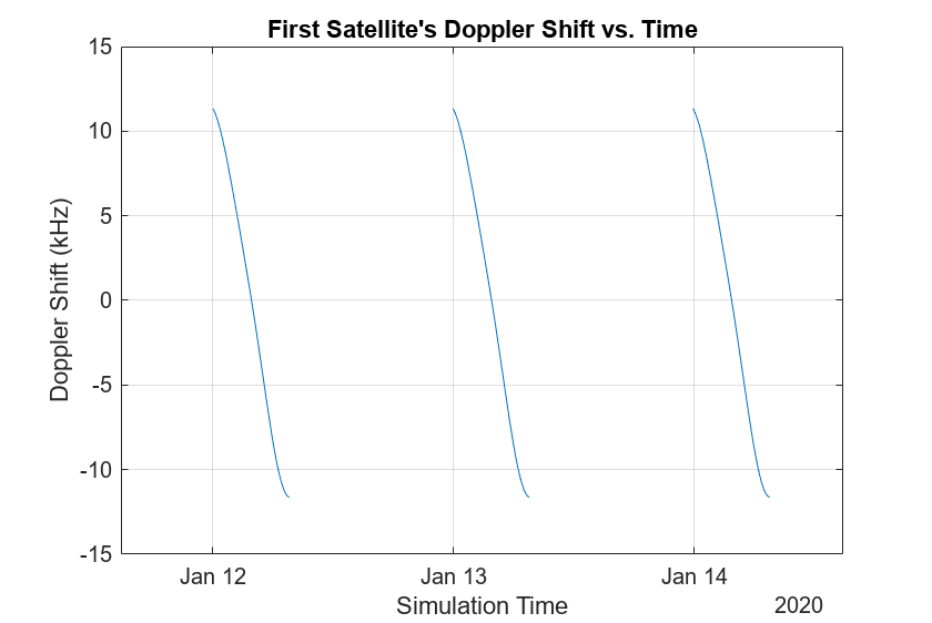
ドップラーシフトとドップラーシフトの変化率を計算する
この例では、5 GHz の C バンド周波数を考慮します。dopplershift 関数を使用してドップラーシフトとドップラーシフトの変化を計算します。
% Emitted carrier frequency in Hz
fc = 5e9;
% Calculate Doppler shift and get additional information about Doppler. The
% Doppler information output contains relative velocity and Doppler rate.
% The dopplershift function internally performs access analysis and returns
% NaN whenever there is no access.
[fShift,time,dopplerInfo] = dopplershift(sat,gs,Frequency=fc);
最初の衛星に対応するドップラーシフトをプロットします。
plot(time,fShift(1,:)/1e3)                        % Plot in kHz
xlim([time(1) time(end)])
title("First Satellite's Doppler Shift vs. Time")
xlabel("Simulation Time")
ylabel("Doppler Shift (kHz)")
grid on
最初の衛星に対応するドップラー率をプロットします。
plot(time(1:end-1),dopplerInfo.DopplerRate(1,:))  % Plot in Hz/s
xlim([time(1) time(end-1)])
title("First Satellite's Doppler Rate vs. Time")
xlabel("Simulation Time")
ylabel("Doppler Rate (Hz/s)")
grid on

最初の衛星の名前と軌道を表示し、12 時間にわたる将来のグラウンド トラック、つまりリードタイムをプロットします。破線黄色は将来のグラウンド トラックを示し、実線黄色は過去のグラウンド トラックを示します。
sat(1).ShowLabel = true;
show(sat(1).Orbit);
groundTrack(sat(1), ...
    LeadTime=12*3600);   % In seconds
campos(v,84,-176,7.3e7);

衛星と地上局を使ったシナリオを再生します。
play(sc)

参考
オブジェクト
関数
orbitalElements|aer|play