rfplot
Plot cumulative RF budget result vs. cascade input frequency and amplifier power characteristics
Description
Use the rfplot function to plot:
Cumulative RF budget result vs. cascade input frequency
Magnitude response of the S-parameters
Amplifier power characteristics (since R2023a)
One-tone and two-tone analysis (since R2023b)
rfplot( plots the magnitude
response of rfobj)S-Parameters, S21 for the
cascaded budget object, rfobj.
rfplot(
plots the RF budget result specified by RF parameters rfobj,rfpara)rfpara
versus a range of input frequencies. The input frequencies are applied to the
cascade of elements in the RF budget object, rfobj.
Cumulative (that is, terminated subcascade) results are automatically computed to show the variation of the RF budget result through the entire design.
rfplot( plots the magnitude
response of rfobj,m,n)S-Parameters, Smn
(S11, S12,
S21 , or S22) for the cascaded
budget object, rfobj.
rfplot( plots the
cumulative RF budget result or amplifier power
characteristics (since R2023a) on the axes specified in ax,___)ax
instead of the current axes. Specify ax as the first input
argument followed by any of the input arguments in the previous syntaxes. Return
the current axes using the gca function.
Examples
Create an RF system.
Create an RF bandpass filter using the Touchstone file RFBudget_RF.
f1 = nport('RFBudget_RF.s2p','RFBandpassFilter');
Create an amplifier with a gain of 11.53 dB, a noise figure (NF) of 1.53 dB, and an output third-order intercept (OIP3) of 35 dBm.
a1 = amplifier(Name="RFAmplifier",Gain=11.53,NF=1.53,OIP3=35);Create a demodulator with a gain of –6 dB, a NF of 4 dB, and an OIP3 of 50 dBm.
d = modulator(Name="Demodulator",Gain=-6,NF=4,OIP3=50, ...
        LO=2.03e9,ConverterType="Down");
Create an IF bandpass filter using the Touchstone file RFBudget_IF.
f2 = nport('RFBudget_IF.s2p','IFBandpassFilter');
Create an amplifier with a gain of 30 dB, a NF of 8 dB, and an OIP3 of 37 dBm.
a2 = amplifier(Name="IFAmplifier",Gain=30,NF=8,OIP3=37);Calculate the RF budget of the system using an input frequency of 2.1 GHz, an input power of –30 dBm, and a bandwidth of 45 MHz.
b = rfbudget([f1 a1 d f2 a2],2.1e9,-30,45e6)
b =
  rfbudget with properties:

               Elements: [1x5 rf.internal.rfbudget.Element]
         InputFrequency: 2.1 GHz
    AvailableInputPower: -30 dBm
        SignalBandwidth:  45 MHz
                 Solver: Friis
             AutoUpdate: true

   Analysis Results
        OutputFrequency: (GHz) [   2.1    2.1   0.07    0.07   0.07]
            OutputPower: (dBm) [-31.53    -20    -26  -27.15  2.847]
         TransducerGain: (dB)  [-1.534  9.996  3.996   2.847  32.85]
                     NF: (dB)  [ 1.533  3.064  3.377   3.611  7.036]
                   IIP3: (dBm) [   Inf     25  24.97   24.97  4.116]
                   OIP3: (dBm) [   Inf     35  28.97   27.82  36.96]
                    SNR: (dB)  [ 65.91  64.38  64.07   63.83  60.41]
Plot the available output power.
rfplot(b,'Pout')
view(90,0)
Plot the transducer gain.
rfplot(b,'GainT')
view(90,0)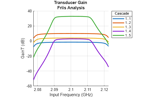
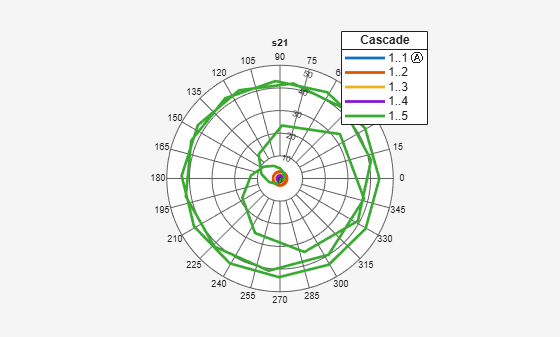
Plot S-parameters of an RF system on a Smith Chart and a Polar plot.
s = smithplot(b,1,1,GridType="ZY"); 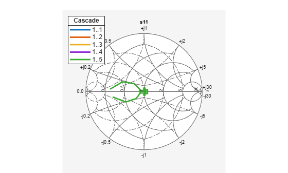
p = polar(b,2,1);
Create an RF bandpass filter using the Touchstone file RFBudget_RF.
f1 = nport('RFBudget_RF.s2p','RFBandpassFilter');
Create an amplifier with a gain of 11.53 dB, a noise figure (NF) of 1.53 dB, and an output third-order intercept (OIP3) of 35 dBm.
a1 = amplifier(Name="RFAmplifier",Gain=11.53,NF=1.53,OIP3=35);Create a demodulator with a gain of –6 dB, a NF of 4 dB, and an OIP3 of 50 dBm.
d = modulator(Name="Demodulator",Gain=-6,NF=4,OIP3=50, ...
        LO=2.03e9,ConverterType="Down");
Create an IF bandpass filter using the Touchstone file RFBudget_IF.
f2 = nport('RFBudget_IF.s2p','IFBandpassFilter');
Create an amplifier with a gain of 30 dB, a NF of 8 dB, and an OIP3 of 37 dBm.
a2 = amplifier(Name='IFAmplifier',Gain=30,NF=8,OIP3=37);Calculate the RF budget of the system using an input frequency of 2.1 GHz, an input power of –30 dBm, and a bandwidth of 45 MHz.
b = rfbudget([f1 a1 d f2 a2],2.1e9,-30,45e6);
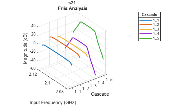
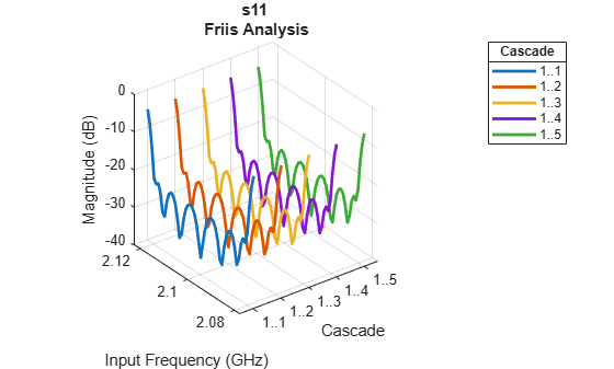
Show the analysis in the RF plot.
rfplot(b)
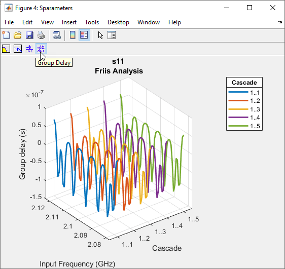
Group Delay
To plot the group delay, first plot the S11 data for the RF System.
rfplot(b,1,1)
Use the Group Delay option on the plot graph to plot the group delay of the RF system.
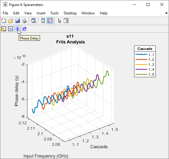
Phase Delay
Use the Phase Delay option on the plot graph to plot the phase delay of the RF System.
Since R2023a
Create an amplifier object.
amp = amplifier;
Plot the amplifier power characteristics at 2.1 GHz.
rfplot(amp,2.1e9)

Set OIP3 of amplifier to 25 dBm.
amp.OIP3 = 25;
Plot the amplifier power characteristics at 2.1 GHz with nonlinearity.
rfplot(amp,2.1e9)

Plot the amplifier power characteristics on the axes specified in ax instead of the current axes.
f = figure;
ax = axes(f);
rfplot(ax,amp,2.1e9)

Since R2023b
One- and two-tone analysis are used to evaluate the performance of nonlinear systems. This example uses a 2-element system with an amplifier, a nonlinear element and a filter.
Define the input frequency, signal power, and signal bandwidth.
freq = 2.1e9;
inputPower = -30;
bandwidth = 10e6;
Create an amplifier with a noise figure of 3 dB and OIP3 of 30 dB.
amp = amplifier(Gain=10, NF=3, OIP3=30);
Create a filter with an input S2P file.
filt = nport('passive.s2p'); Create an rfbudget object with amplifier and filter element to model a two-element chain.
rfobj = rfbudget(Elements=[amp filt], Solver="HarmonicBalance", ...
                 InputFrequency=freq, ...
                 AvailableInputPower=inputPower, ...
                 SignalBandwidth=bandwidth);
Plot the one-tone analysis of the system. Use the one-tone plot to determine the presence of harmonics in the output.
rfplot(rfobj,'OneTone');
Plot the two-tone analysis of the system. Use the two-tone analysis plot to evaluate intermodulation distortion or products of the RF components.
rfplot(rfobj,'TwoTone');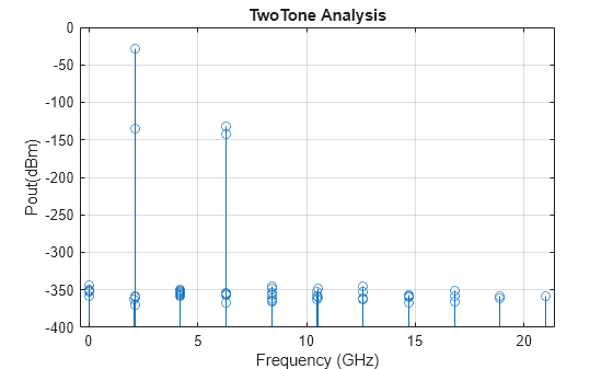
Zoom-in the frequency of interest in the two-tone analysis plot to evaluate the intermodulation distortion (products).
rfplot(rfobj,'TwoTone');
axis([2.09,2.15,-360,-40])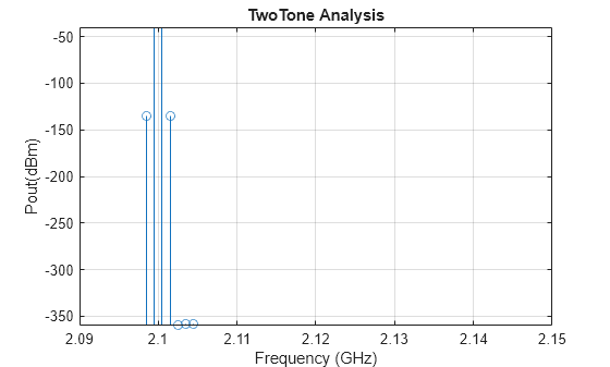
Input Arguments
Version History
Introduced in R2017bSee Also
rfbudget | show | computeBudget | exportScript | exportRFBlockset | exportTestbench | rfplot | smithplot | polar