Train Hybrid-Action PPO Agent for Path-Following Control

This example demonstrates how to train a hybrid-action Proximal Policy Optimization (PPO) agent to perform path-following control (PFC) for a vehicle. A hybrid action agent is an Reinforcement Learning (RL) agent that has an action space consisting of both discrete and continuous actions. For an example showing how to use a hybrid-action SAC agent, see Train Hybrid SAC Agent for Path-Following Control. For an example that shows how to use two RL agents (one with discrete action space, the other with continuous action space), see Train Multiple Agents for Path Following Control. In that example, a DDPG agent provides continuous acceleration values for the longitudinal control loop while a DQN agent provides discrete steering angle values for the lateral control loop.

Overview

A PFC system controls the vehicle under consideration (also referred as "ego vehicle") such that it:

• Maintains a given traveling speed

• Maintains a safe distance from a vehicle in front of it, also called lead vehicle, by controlling longitudinal acceleration and braking

• Travels along the centerline of its lane by controlling the front steering angle

For more information, see Path Following Control System (Model Predictive Control Toolbox).

In this example, you train a single hybrid-action PPO agent to control both the lateral steering (discrete action) and the longitudinal speed (continuous action) of the ego vehicle.

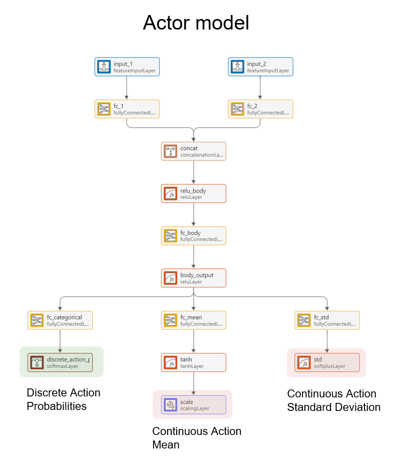
The actor approximation model has three outputs:

1. The categorical distribution output — A vector of probabilities for a discrete action.

2. The mean values output — A vector of mean values of Gaussian distributions, each for each continuous action dimension.

3. The standard deviation values output — A vector of standard deviations of those Gaussian distributions.

The actor samples actions as follows:

1. Discrete part of the action: A discrete value sampled among the possible values, according to the probabilities expressed by the categorical distribution output of the approximation model.

2. Continuous part of the action: Continuous values sampled according to the Gaussian distributions expressed by the mean and standard deviation outputs of the approximation model.

The image below shows the actor model used in this example.

For more information on the hybrid-action PPO algorithm, see Proximal Policy Optimization (PPO) Agent.

Fix Random Number Stream for Reproducibility

The example code might involve computation of random numbers at several stages. Fixing the random number stream at the beginning of some sections in the example code preserves the random number sequence in the section every time you run it, which increases the likelihood of reproducing the results. For more information, see Results Reproducibility.

Fix the random number stream with seed 0 and random number algorithm Mersenne twister. For more information on controlling the seed used for random number generation, see rng.

previousRngState = rng(0,"twister");

The output previousRngState is a structure that contains information about the previous state of the stream. You will restore the state at the end of the example.

Create Environment Object

The environment for this example includes a simple bicycle model for the ego vehicle and a simple longitudinal model for the lead vehicle. The agent controls the longitudinal acceleration, braking, and the front steering angle of the ego vehicle.

Load the environment parameters.

HPPOPFCParams

Open the Simulink® model.

mdl = "HPPOPFC";
open_system(mdl)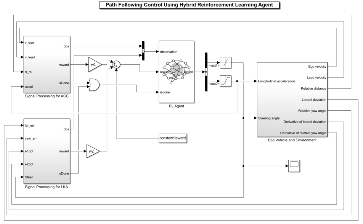

The simulation terminates if any of the following conditions occur.

• $|e_1|>1$ — The magnitude of the lateral deviation is greater than 1.

• $$V_{ego}<0.5$$— The longitudinal velocity of the ego vehicle is less than 0.5.

• $$D_{rel}<0$$ — The distance between the ego and the lead vehicle is less than zero.

To determine the ego vehicle's reference velocity$$V_{ref}$$:

• The safe distance is a linear function of the ego vehicle's longitudinal velocity $V$. That is, $$t_{gap}*V+D_{default}$$.

• If the relative distance is less than the safe distance, the ego vehicle tracks the minimum value between the velocity of the lead vehicle and the desired velocity set by the driver. Setting the reference velocity in this way allows the ego vehicle to maintain a safe distance from the lead vehicle. If the relative distance is greater than the safe distance, the ego vehicle uses the desired velocity set by the driver as the reference velocity.

Observation:

• The first observation channel contains the longitudinal measurements. These are the velocity error $$e_V=V_{ref}-V$$, its integral $$\int e$$, and the ego vehicle longitudinal velocity $V$.

• The second observation channel contains the lateral measurements. These are the lateral deviation $e_1$, the relative yaw angle $e_2$(the yaw angle error with respect to the lane centerline), their derivatives $${\underset{}{\overset{\dot{}}{e}}}_1$$ and $${\underset{}{\overset{\dot{}}{e}}}_2$$, and their integrals $\int e_1$ and $\int e_2$.

Action:

• The discrete action $a_t$ — The action signal consists of discrete steering angle actions which take values from –15 degrees (–0.2618 rad) to 15 degrees (0.2618 rad) in steps of 1 degree (0.0175 rad).

• The continuous action $$u_t$$ — The action signal consists of continuous acceleration values between –3 and 2 $m/s^2$.

Reward:

• The reward $r_t$, provided at every time step $t$, is the weighted sum of the reward $r_{\text{lateral}}$ for the lateral control, the reward $r_{\text{longitudinal}}$ for the longitudinal control, and the constant reward $r_{\text{everystep}}$.

$$\begin{array}{l}{r}_t=w_1{r}_{lateral}+w_2{r}_{longitudinal}+r_{everystep}\\ r_{lateral}=-(0.1e_1^2+0.5u_{t-1}^2)-100F_t+2H_t\\ r_{longitudinal}=-(0.01e_V^2+0.1a_{t-1}^2)-100F_t+M_t\\ w_1=1/50\\ w_2=1/120\\ r_{everystep}=1/10\end{array}$$

In these equations, $$u_{t-1}$$ is the steering input from the previous time step, $a_{t-1}$ is the acceleration input from the previous time step, and:

• $F_t=1$ if the simulation terminates, otherwise $F_t=0$.

• $M_t=1$ if $e_V^2<1$, otherwise $M_t=0$.

• $H_t=1$if $e_1^2<0.01$, otherwise $H_t=0$.

The logical terms in the reward functions ($F_t$, $M_t$, and $H_t$) penalize the agent if the simulation terminates early, while encouraging the agent to make both the lateral error and velocity error small.

Create the observation specification. Because an observation contains multiple channels in this Simulink environment, you must use the bus2RLSpec function to create the specification. For more information about Simulink environments, see Create Custom Simulink Environments.

Create a bus object.

obsBus = Simulink.Bus();

Add the first bus element.

obsBus.Elements(1) = Simulink.BusElement;
obsBus.Elements(1).Name = "signal1";
obsBus.Elements(1).Dimensions = [3,1];

Add the second bus element.

obsBus.Elements(2) = Simulink.BusElement;
obsBus.Elements(2).Name = "signal2";
obsBus.Elements(2).Dimensions = [6,1];

Create the observation specification.

obsInfo= bus2RLSpec("obsBus");

Create the action specification. For the hybrid-action PPO agent, you must have two action channels. The first action channel must be for the discrete part of the action, and the second must be for the continuous part of the action. Use the bus2RLSpec function to create the specification, as for the observation specification case.

Create a bus object.

actBus = Simulink.Bus();

Add the first bus element for the discrete part of the action. The discrete part of the action must be the first action channel.

actBus.Elements(1) = Simulink.BusElement;
actBus.Elements(1).Name = "act1";

Add the second bus element for the continuous part of the action.

actBus.Elements(2) = Simulink.BusElement;
actBus.Elements(2).Name = "act2";
actBus.Elements(2).Dimensions = [1,1];
actInfo = bus2RLSpec("actBus","DiscreteElements", ...
           {"act1",(-15:15)*pi/180});

Define the limits of continuous actions.

actInfo(2).LowerLimit = -3;
actInfo(2).UpperLimit = 2;

Create a Simulink environment object, specifying the block paths for the agent block. For more information, see rlSimulinkEnv.

blks = mdl + "/RL Agent";
env = rlSimulinkEnv(mdl,blks,obsInfo,actInfo);

Specify a reset function for the environment by using its ResetFcn property. The function pfcResetFcn (provided at the end of the example) sets the initial conditions of the lead and ego vehicles at the beginning of every episode during training.

env.ResetFcn = @pfcResetFcn;

Create Hybrid-Action PPO Agent

Fix the random number stream.

rng(0, "twister");

Set the sample time, in seconds, for the Simulink model and the RL agent object.

Ts = 0.1;

Set the simulation time, in seconds.

Tf = 60;

Create a default hybrid-action PPO agent. When the action specification defines a hybrid action space (that is, an action space that contains both a discrete and a continuous action channel), rlPPOAgent creates a hybrid-action PPO agent. The hybrid-action PPO agent uses rlHybridStochasticActor as the actor and rlValueFunction as the critic.

agent = rlPPOAgent(obsInfo, actInfo);

Specify the agent options:

• Set the mini-batch size to 512 to make the training more stable.

• The default LearningFrequency is -1, meaning that the PPO agent collects at least 10*MiniBatchSize experiences and updates the agent at the end of the episode.

• Set learning rate to 1e-3 for the actor and the critics.

• Set gradient thresholds to 1 to limit the gradient values.

• Set the normalized advantage method to "current" for more stable training.

agent.SampleTime = Ts;
agent.AgentOptions.MiniBatchSize = 512;
agent.AgentOptions.ExperienceHorizon = Tf/Ts;
agent.AgentOptions.ActorOptimizerOptions.LearnRate = 1e-3;
agent.AgentOptions.ActorOptimizerOptions.GradientThreshold = 1;
agent.AgentOptions.CriticOptimizerOptions.LearnRate = 1e-3;
agent.AgentOptions.CriticOptimizerOptions.GradientThreshold = 1;
agent.AgentOptions.NormalizedAdvantageMethod = "current";

Set the entropy loss weights for the discrete and continuous actions. The first element is for discrete actions and the second element is for continuous actions.

agent.AgentOptions.EntropyLossWeight= [0.001, 0.001];

Train Hybrid-Action PPO Agent

Specify the training options. For this example, use the following options.

• Run each training episode for a maximum of 15000 episodes, with each episode lasting a maximum of maxsteps time steps.

• Display the training progress in the Reinforcement Learning Training Monitor dialog box.

• Stop the training when the agent receives an average evaluation episode reward greater than 79.6.

• Use parallel training for more efficient training when parallel computing resources are available.

• To improve performance, do not save the simulation data during training. To save the simulation data during training instead, set SimulationStorageType to "file" or "memory".

maxepisodes = 15000;
maxsteps = ceil(Tf/Ts);
trainingOpts = rlTrainingOptions( ...        
    MaxEpisodes=maxepisodes, ...
    MaxStepsPerEpisode=maxsteps, ...
    StopTrainingCriteria="EvaluationStatistic", ...
    StopTrainingValue=79.6, ...
    UseParallel=canUseParallelPool,...
    SimulationStorageType="none");

Fix the random number stream.

rng(0, "twister");

Train the agent by using the train function. Training the agent is a computationally intensive process. To save time while running this example, load a pretrained agent by setting doTraining to false. To train the agent yourself, set doTraining to true.

doTraining = false;
if doTraining    
    % Evaluate the agent after every 25 training episodes. 
    % The evaluation statistic is the mean value of 
    % the statistic over five evaluation episodes.    
    evaluator = rlEvaluator(EvaluationFrequency=25, ...
        NumEpisodes=5, RandomSeeds=101:105);

    % Train the agent.
    trainingStats = train(agent,env,trainingOpts,Evaluator=evaluator);
else
    % Load the pretrained agent for the example.
    load("rlHybridPPOPFCAgent.mat")       
end

This figure shows a snapshot of the training progress.

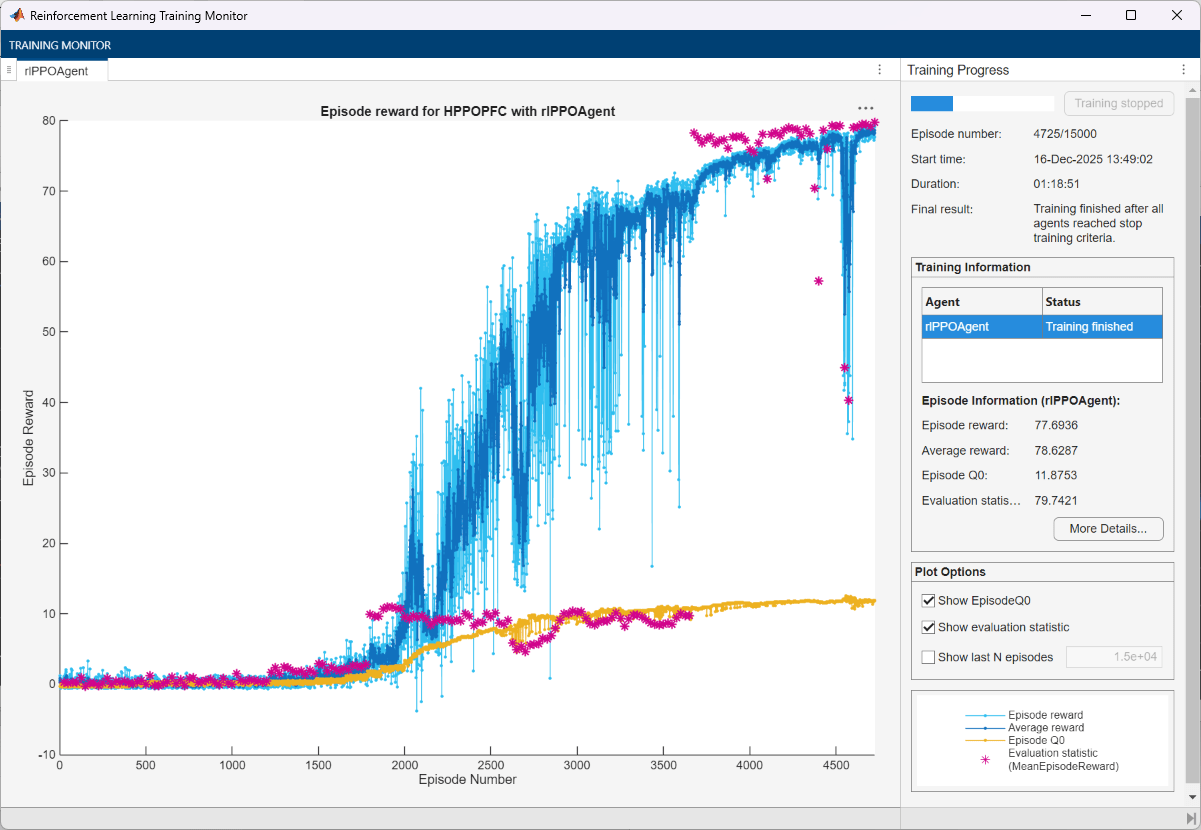
The training converges before 5000 episodes.

Simulate the Trained PPO Agent

Fix the random number stream.

rng(0, "twister");

By default, the agent uses a greedy (hence deterministic) policy in simulation. To use the exploratory policy instead, set the UseExplorationPolicy agent property to true.

To validate the performance of the trained agent, simulate the agent within the Simulink environment. For more information on agent simulation, see rlSimulationOptions and sim.

simOptions = rlSimulationOptions(MaxSteps=maxsteps);
experience = sim(env,agent,simOptions);

To validate the trained agent using deterministic initial conditions, simulate the model in Simulink. In this example, the lead vehicle is 70 m ahead of the ego vehicle at the beginning of the simulation.

e1_initial = -0.4;
e2_initial = 0.1;
x0_lead = 70;
sim(mdl)

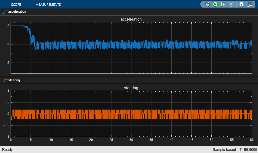
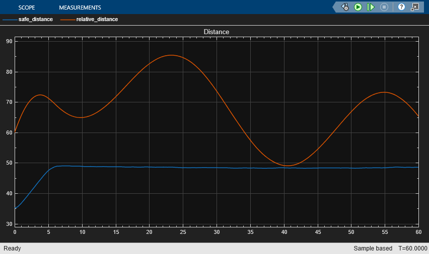
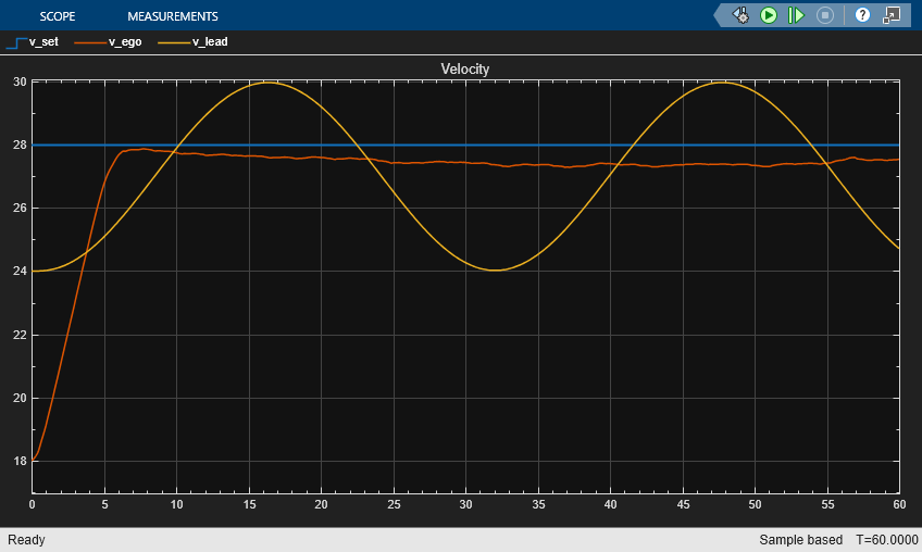
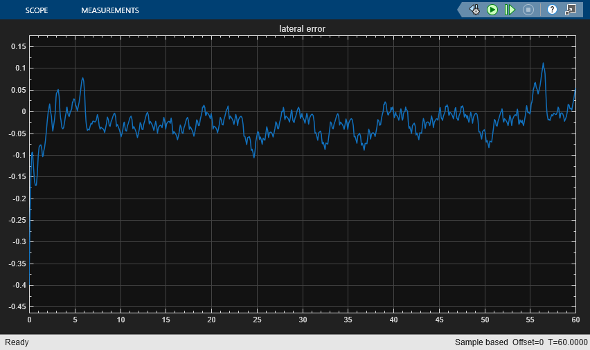
The plots show the results:

• The lead vehicle changes speed from 24 m/s to 30 m/s periodically (see the velocity plot).

• From 0 to 6 seconds, the ego vehicle tracks the set velocity (see the velocity plot) and experiences significant acceleration (see the acceleration and steering plot). After that, the acceleration becomes small.

• The lateral deviation decreases greatly within 1 second and remains less than 0.1 m (see the lateral error plot).

• The ego vehicle maintains a safe distance throughout the simulation (see the distance plot).

Restore the random number stream using the information stored in previousRngState.

rng(previousRngState)

Environment Reset Function

The reset function pfcResetFcn sets the initial conditions of the lead and ego vehicles at the beginning of every episode during training. The sim function calls the reset function at the start of each simulation episode, and the train function calls it at the start of each training episode. The reset function takes as input, and returns as output, a Simulink.SimulationInput (Simulink) object. The output object specifies temporary changes applied to the model, which are then discarded when the simulation or training completes.

For this example, the reset function uses the setVariable (Simulink) function to set variables in the model workspace. For more information, see Reset Function for Simulink Environments.

function in = pfcResetFcn(in)

    % random value for initial position of lead vehicle
    in = setVariable(in,'x0_lead',40+randi(60,1,1));

    % random value for lateral deviation
    in = setVariable(in,'e1_initial', 0.5*(-1+2*rand));

    % random value for relative yaw angle
    in = setVariable(in,'e2_initial', 0.1*(-1+2*rand));

end