シミュレーション データを使用した複数クラス故障検出
この例では、Simulink® モデルを使用して故障データと健全データを生成する方法を説明します。このデータを使用して、さまざまな故障の組み合わせを検出する複数クラス分類器を開発します。この例は 3 重往復ポンプ モデルを使用し、漏れ、閉塞、およびベアリングの故障を含みます。
モデルの設定
この例では、zip ファイルに保存されている多くのサポート ファイルを使用します。ファイルを解凍してサポート ファイルにアクセスし、モデル パラメーターを読み込みます。
unzip('pdmRecipPump_supportingfiles.zip')

% Load Parameters
pdmRecipPump_Parameters %Pump
CAT_Pump_1051_DataFile_imported %CAD
往復ポンプ モデル
往復ポンプは、電気モーター、ポンプ ハウジング、ポンプ クランク、およびポンプ プランジャーで構成されています。
mdl = 'pdmRecipPump';
open_system(mdl)
open_system([mdl,'/Pump'])
ポンプ モデルは、シリンダーの漏れ、吸込口の閉塞、およびベアリング摩擦の増加という 3 タイプの故障をモデル化するように設定されます。これらの故障はワークスペース変数としてパラメーター化され、ポンプ ブロック ダイアログによって設定されます。

故障データと健全データのシミュレーション
3 つの故障タイプそれぞれについて、故障なしから重大な故障までの故障重大度を表す値の配列を作成します。
% Define fault parameter variations
numParValues = 10;
leak_area_set_factor = linspace(0.00,0.036,numParValues);
leak_area_set = leak_area_set_factor*TRP_Par.Check_Valve.In.Max_Area;
leak_area_set = max(leak_area_set,1e-9); % Leakage area cannot be 0
blockinfactor_set = linspace(0.8,0.53,numParValues);
bearingfactor_set = linspace(0,6e-4,numParValues);
ポンプ モデルはノイズを含めるように設定されているため、同じ故障パラメーター値でモデルを実行すると、結果としてさまざまなシミュレーション出力が得られます。これは、同じ故障状態と重大度に対して複数のシミュレーション結果が可能であることを意味するので、分類器の開発に役立ちます。そのような結果が得られるシミュレーションを設定するには、故障パラメーター値のベクトルを作成します。ここで値は、故障なし、1 つの故障、2 つの故障の組み合わせ、および 3 つの故障の組み合わせを表します。故障なし、1 つの故障、などの各グループについて、上記で定義されている故障パラメーター値から、故障値の 125 の組み合わせを作成します。これにより故障パラメーター値の合計 1000 の組み合わせが得られます。これら 1000 のシミュレーションを並列で実行する場合、標準のデスクトップでは約 1 時間かかり、約 620 MB のデータが生成されることに注意してください。シミュレーション時間を短縮させるには、runAll = true を runAll = false に変更して、故障の組み合わせの数を 20 に減らします。データセットが大きいほど、よりロバストな分類器となることに注意してください。
% Set number of elements in each fault group
runAll = true;
if runAll
    % Create a large dataset to build a robust classifier
    nPerGroup = 100;
else
    % Create a smaller dataset to reduce simulation time
    nPerGroup = 20; %#ok<UNRCH>
end

rng('default');    % Feed default seed to rng (Random number generator)

% No fault simulations
leakArea = repmat(leak_area_set(1),nPerGroup,1);
blockingFactor = repmat(blockinfactor_set(1),nPerGroup,1);
bearingFactor = repmat(bearingfactor_set(1),nPerGroup,1);

% Single fault simulations
idx = ceil(10*rand(nPerGroup,1));
leakArea = [leakArea; leak_area_set(idx)'];
blockingFactor = [blockingFactor;repmat(blockinfactor_set(1),nPerGroup,1)];
bearingFactor = [bearingFactor;repmat(bearingfactor_set(1),nPerGroup,1)];
idx = ceil(10*rand(nPerGroup,1));
leakArea = [leakArea; repmat(leak_area_set(1),nPerGroup,1)];
blockingFactor = [blockingFactor;blockinfactor_set(idx)'];
bearingFactor = [bearingFactor;repmat(bearingfactor_set(1),nPerGroup,1)];
idx = ceil(10*rand(nPerGroup,1));
leakArea = [leakArea; repmat(leak_area_set(1),nPerGroup,1)];
blockingFactor = [blockingFactor;repmat(blockinfactor_set(1),nPerGroup,1)];
bearingFactor = [bearingFactor;bearingfactor_set(idx)'];

% Double fault simulations
idxA = ceil(10*rand(nPerGroup,1));
idxB = ceil(10*rand(nPerGroup,1));
leakArea = [leakArea; leak_area_set(idxA)'];
blockingFactor = [blockingFactor;blockinfactor_set(idxB)'];
bearingFactor = [bearingFactor;repmat(bearingfactor_set(1),nPerGroup,1)];
idxA = ceil(10*rand(nPerGroup,1));
idxB = ceil(10*rand(nPerGroup,1));
leakArea = [leakArea; leak_area_set(idxA)'];
blockingFactor = [blockingFactor;repmat(blockinfactor_set(1),nPerGroup,1)];
bearingFactor = [bearingFactor;bearingfactor_set(idxB)'];
idxA = ceil(10*rand(nPerGroup,1));
idxB = ceil(10*rand(nPerGroup,1));
leakArea = [leakArea; repmat(leak_area_set(1),nPerGroup,1)];
blockingFactor = [blockingFactor;blockinfactor_set(idxA)'];
bearingFactor = [bearingFactor;bearingfactor_set(idxB)'];

% Triple fault simulations
idxA = ceil(10*rand(nPerGroup,1));
idxB = ceil(10*rand(nPerGroup,1));
idxC = ceil(10*rand(nPerGroup,1));
leakArea = [leakArea; leak_area_set(idxA)'];
blockingFactor = [blockingFactor;blockinfactor_set(idxB)'];
bearingFactor = [bearingFactor;bearingfactor_set(idxC)'];
故障パラメーターの組み合わせを使用して Simulink.SimulationInput オブジェクトを作成します。各シミュレーション入力につき、異なる結果が生成されるようにランダム シードを必ず異なる値に設定します。
for ct = numel(leakArea):-1:1
    simInput(ct) = Simulink.SimulationInput(mdl);
    simInput(ct) = setVariable(simInput(ct),'leak_cyl_area_WKSP',leakArea(ct));
    simInput(ct) = setVariable(simInput(ct),'block_in_factor_WKSP',blockingFactor(ct));
    simInput(ct) = setVariable(simInput(ct),'bearing_fault_frict_WKSP',bearingFactor(ct));
    simInput(ct) = setVariable(simInput(ct),'noise_seed_offset_WKSP',ct-1);
end
関数 generateSimulationEnsemble を使用して、上で定義された Simulink.SimulationInput オブジェクトによって定義されるシミュレーションを実行し、ローカル サブフォルダーに結果を格納します。次に、格納された結果から simulationEnsembleDatastore を作成します。
% Run the simulation and create an ensemble to manage the simulation
% results

if isfolder('./Data')
    % Delete existing mat files
    delete('./Data/*.mat')
end

[ok,e] = generateSimulationEnsemble(simInput,fullfile('.','Data'),'UseParallel',false,'ShowProgress',false);    %Set the UseParallel flag to true to use parallel computing capabilities
ens = simulationEnsembleDatastore(fullfile('.','Data'));
シミュレーション結果からの特徴の処理と抽出
このモデルはポンプの吐出圧力、出流量、モーター速度、およびモーター電流をログに記録するよう設定されます。
ens.DataVariables
ans = 8×1 string array
    "SimulationInput"
    "SimulationMetadata"
    "iMotor_meas"
    "pIn_meas"
    "pOut_meas"
    "qIn_meas"
    "qOut_meas"
    "wMotor_meas"
アンサンブルのメンバーごとに、ポンプ出流量を前処理し、ポンプ出流量に基づいて状態インジケーターを計算します。状態インジケーターは後で故障分類のために使用されます。前処理のため、出流量の最初の 0.8 秒を削除します。これにはシミュレーションおよびポンプ始動からの過渡状態が含まれるためです。前処理の一部として、出流量のパワー スペクトルを計算し、SimulationInput を使って故障変数の値を返します。
対象とする変数だけが読み取りで返されるようにアンサンブルを設定し、この例の最後で定義されている関数 preprocess を呼び出します。
ens.SelectedVariables = ["qOut_meas", "SimulationInput"];
reset(ens)
data = read(ens)
data=1×2 table
    2001×1 timetable    1×1 SimulationInput
[flow,flowP,flowF,faultValues] = preprocess(data);
流量と流量スペクトルをプロットします。プロットされるデータは故障なしの状態のものです。
% Figure with nominal
subplot(211);
plot(flow.Time,flow.Data);
subplot(212);
semilogx(flowF,pow2db(flowP));
xlabel('Hz')

流量スペクトルは、期待された周波数での共振ピークを示しています。具体的には、ポンプのモーター速度は 950 rpm、つまり 15.833 Hz であり、ポンプはシリンダーを 3 つもつため、流量は 3*15.833 Hz つまり 47.5 Hz で基本波であり、47.5 Hz の倍数において高調波であると予想されます。流量スペクトルは、期待される共振ピークを明確に示しています。ポンプの 1 つのシリンダーに故障が生じると、ポンプのモーター速度 15.833 Hz およびその高調波で共振が発生します。
流量スペクトルおよび低速信号は、可能な状態インジケーターをある程度示唆しています。具体的には、平均や分散などの一般的な信号統計量、およびスペクトル特性です。ピーク振幅の周波数、15.833 Hz 周辺のエネルギー、47.5 Hz 周辺のエネルギー、および 100 Hz を超えるエネルギーなどの、期待される高調波に関連するスペクトル状態インジケーターが計算されます。スペクトル尖度ピークの周波数も計算されます。
状態インジケーターのデータ変数および故障変数値の状態変数を使用して、アンサンブルを設定します。その後、関数 extractCI を呼び出して特徴を計算し、writeToLastMemberRead コマンドを使用して特徴および故障変数の値をアンサンブルに追加します。関数 extractCI はこの例の最後で定義されています。
ens.DataVariables = [ens.DataVariables; ...
    "fPeak"; "pLow"; "pMid"; "pHigh"; "pKurtosis"; ...
    "qMean"; "qVar"; "qSkewness"; "qKurtosis"; ...
    "qPeak2Peak"; "qCrest"; "qRMS"; "qMAD"; "qCSRange"];
ens.ConditionVariables = ["LeakFault","BlockingFault","BearingFault"];

feat = extractCI(flow,flowP,flowF);
dataToWrite = [faultValues, feat];
writeToLastMemberRead(ens,dataToWrite{:})
上記のコードは、シミュレーション アンサンブルの最初のメンバーの状態インジケーターを前処理して計算します。アンサンブルの hasdata コマンドを使用して、アンサンブルのすべてのメンバーについてこれを繰り返します。さまざまな故障状態下におけるシミュレーション結果を把握するには、アンサンブルを 100 要素ごとにプロットします。
%Figure with nominal and faults
figure,
subplot(211);
lFlow = plot(flow.Time,flow.Data,'LineWidth',2);
subplot(212);
lFlowP = semilogx(flowF,pow2db(flowP),'LineWidth',2);
xlabel('Hz')
ct = 1;
lColors = get(lFlow.Parent,'ColorOrder');
lIdx = 2;

% Loop over all members in the ensemble, preprocess
% and compute the features for each member
while hasdata(ens)

    % Read member data
    data = read(ens);

    % Preprocess and extract features from the member data
    [flow,flowP,flowF,faultValues] = preprocess(data);
    feat = extractCI(flow,flowP,flowF);

    % Add the extracted feature values to the member data
    dataToWrite = [faultValues, feat];
    writeToLastMemberRead(ens,dataToWrite{:})

    % Plot member signal and spectrum for every 100th member
    if mod(ct,100) == 0
        line('Parent',lFlow.Parent,'XData',flow.Time,'YData',flow.Data, ...
            'Color', lColors(lIdx,:));
        line('Parent',lFlowP.Parent,'XData',flowF,'YData',pow2db(flowP), ...
            'Color', lColors(lIdx,:));
        if lIdx == size(lColors,1)
            lIdx = 1;
        else
            lIdx = lIdx+1;
        end
    end
    ct = ct + 1;
end
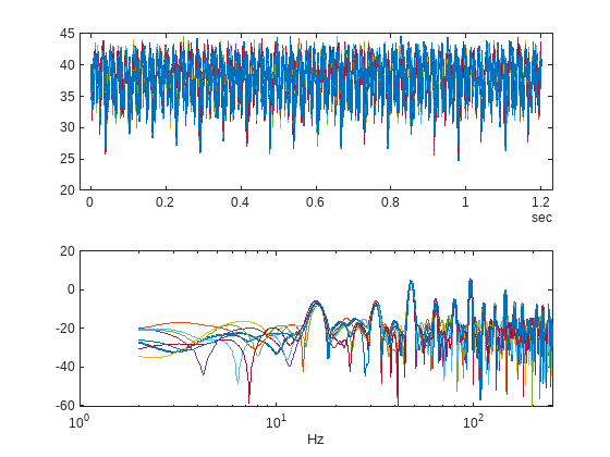
さまざまな故障状態および重大度の下において、期待される周波数でスペクトルに高調波が含まれることに注意してください。
ポンプの故障の検出と分類
前の節では、シミュレーション アンサンブルの全メンバーの流量信号から状態インジケーターを前処理して計算しました。これはさまざまな故障の組み合わせと重大度によるシミュレーション結果に対応します。状態インジケーターを使用して、ポンプの流量信号からポンプの故障を検出し分類することができます。
状態インジケーターを読み取るようにシミュレーション アンサンブルを設定し、tall コマンドと gather コマンドを使用してすべての状態インジケーターと故障変数値をメモリに読み込みます。
% Get data to design a classifier.
reset(ens)
ens.SelectedVariables = [...
    "fPeak","pLow","pMid","pHigh","pKurtosis",...
    "qMean","qVar","qSkewness","qKurtosis",...
    "qPeak2Peak","qCrest","qRMS","qMAD","qCSRange",...
    "LeakFault","BlockingFault","BearingFault"];
idxLastFeature = 14;

% Load the condition indicator data into memory
data = gather(tall(ens));
Evaluating tall expression using the Local MATLAB Session:
- Pass 1 of 1: Completed in 1 min 23 sec
Evaluation completed in 1 min 23 sec
data(1:10,:)
ans=10×17 table
    95.7495      7.4377     96.2464    92.6167    360.9272    38.0157    11.8755    -0.7097    2.9885    19.8385    1.1672    38.1715    2.8614    4.5617e+04    1.0000e-09    0.8000    0
    95.8100      8.7548     76.5278    81.5845    313.7417    38.0201    11.2432    -0.6621    2.8867    19.5544    1.1741    38.1676    2.7860    4.5624e+04    1.0000e-09    0.8000    0
    95.8100      9.3164     95.7408    81.7604    278.1457    38.0174    11.4135    -0.6577    2.8446    17.9044    1.1493    38.1671    2.8103    4.5622e+04    1.0000e-09    0.8000    0
    15.9292    229.8878    172.7189    62.2431    197.8477    35.7389    17.3609    -0.2123    2.2656    19.2586    1.2256    35.9808    3.4465    4.2892e+04    3.2000e-06    0.8000    0
    15.9292    308.9532    176.5983    47.4726    197.8477    35.4528    19.3943    -0.1490    2.1681    19.7606    1.2302    35.7251    3.6708    4.2547e+04    3.6000e-06    0.8000    0
    95.8100     13.8458    112.0437    80.0695    118.3775    37.7084    11.6628    -0.6497    2.8764    19.1244    1.1707    37.8626    2.8293    4.5249e+04    4.0000e-07    0.8000    0
    15.9292    281.9551    180.2683    49.5348    246.6887    35.4056    19.3500    -0.1409    2.1397    18.9874    1.2178    35.6776    3.6818    4.2491e+04    3.6000e-06    0.8000    0
    47.9057    130.4723    147.4706    66.1973    152.3179    36.2711    14.6072    -0.2669    2.3759    17.6148    1.1962    36.4718    3.1342    4.3527e+04    2.4000e-06    0.8000    0
    95.8100      7.1699     98.4639    92.3777    186.2583    38.0051    11.5754    -0.7026    2.8724    18.1011    1.1548    38.1570    2.8239    4.5608e+04    1.0000e-09    0.8000    0
    95.8100     19.4548    107.2855    73.2091    410.5960    37.4699    11.3994    -0.5232    2.4842    16.9398    1.1691    37.6216    2.8115    4.4964e+04    8.0000e-07    0.8000    0
アンサンブル メンバーごとの故障変数値 (データ テーブルの 1 行) を故障フラグに変換し、これらの故障フラグを、各メンバーのさまざまな故障ステータスを捕捉する 1 つのフラグに組み合わせることが可能です。
% Convert the fault variable values to flags
data.LeakFlag = data.LeakFault > 1e-6;
data.BlockingFlag = data.BlockingFault < 0.8;
data.BearingFlag = data.BearingFault > 0;
data.CombinedFlag = data.LeakFlag+2*data.BlockingFlag+4*data.BearingFlag;
状態インジケーターを入力として受け取り、組み合わせた故障フラグを返す分類器を作成します。2 次多項式カーネルを使用するサポート ベクター マシンを学習させます。cvpartition コマンドを使用して、アンサンブルのメンバーを学習用のセットと検証用のセットに分割します。
rng('default') % for reproducibility
predictors = data(:,1:idxLastFeature);
response = data.CombinedFlag;
cvp = cvpartition(size(predictors,1),'KFold',5);

% Create and train the classifier
template = templateSVM(...
    'KernelFunction', 'polynomial', ...
    'PolynomialOrder', 2, ...
    'KernelScale', 'auto', ...
    'BoxConstraint', 1, ...
    'Standardize', true);
combinedClassifier = fitcecoc(...
    predictors(cvp.training(1),:), ...
    response(cvp.training(1),:), ...
    'Learners', template, ...
    'Coding', 'onevsone', ...
    'ClassNames', [0; 1; 2; 3; 4; 5; 6; 7]);
検証データを使用して学習後の分類器の性能をチェックし、結果を混同プロットにプロットします。
% Check performance by computing and plotting the confusion matrix
actualValue = response(cvp.test(1),:);
predictedValue = predict(combinedClassifier, predictors(cvp.test(1),:));
confdata = confusionmat(actualValue,predictedValue);
figure,
labels = {'None', 'Leak','Blocking', 'Leak & Blocking', 'Bearing', ...
    'Bearing & Leak', 'Bearing & Blocking', 'All'};
h = heatmap(confdata, ...
    'YLabel', 'Actual leak fault', ...
    'YDisplayLabels', labels, ...
    'XLabel', 'Predicted fault', ...
    'XDisplayLabels', labels, ...
    'ColorbarVisible','off');
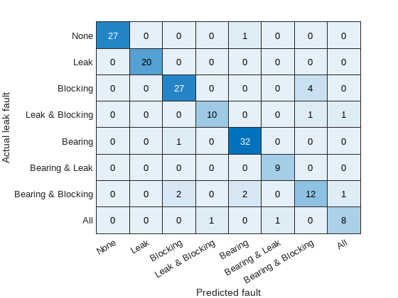
混同プロットは、故障の各組み合わせにつき、故障の組み合わせが正しく予測された回数 (プロットの対角エントリ) と、故障の組み合わせが誤って予測された回数 (非対角エントリ) を示しています。
混同プロットから、分類器は一部の故障状態を正しく分類しなかった (非対角項) ことがわかります。しかし、全体的な検証精度は 90% で、故障があることを予測する精度は 100% です。
% Compute the overall accuracy of the classifier
sum(diag(confdata))/sum(confdata(:))
ans = 0.9062
% Compute the accuracy of the classifier at predicting
% that there is a fault
1-sum(confdata(2:end,1))/sum(confdata(:))
ans =
1
故障が誤って予測されたケースについて調べます。検証データで、実際の故障が閉塞故障でありながら、ベアリングの故障と閉塞故障であると予測されたケースを見つけます。
vData = data(cvp.test(1),:);
b1 = ((actualValue==2) & (predictedValue==6));
fData = vData(b1,15:17)
fData=4×3 table
    1.0000e-09    0.5300    0
    4.0000e-07    0.5900    0
    8.0000e-07    0.7100    0
    4.0000e-07    0.5900    0
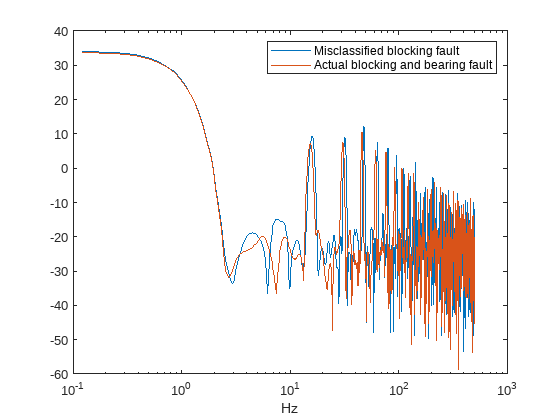
閉塞故障のみが存在する場合に、ベアリングの故障と閉塞故障の両方が予測されたケースを調べてみると、漏れ故障値がノミナル値 1e-9 に近く、閉塞故障値が約 0.6、ベアリング故障値がノミナル値 0 である場合に生じることが明らかになります。故障の誤分類があるケースと実際の故障 (ベアリングと閉塞の両方) があるケースのスペクトルをプロットすると、スペクトルがよく似ているために検出が困難になることがわかります。追加のポンプ測定値を使用してさらに多くの情報を提供することにより、小さな閉塞故障を検出できるように機能を改善することができます。あるいは、特定の周波数帯域のエネルギーを調べる特徴を調査することで、性能を向上させることもできます。
% Configure the ensemble to only read the flow and fault variable values
ens.SelectedVariables = ["qOut_meas","LeakFault","BlockingFault","BearingFault"];
reset(ens)

% Load the ensemble member data into memory
data = gather(tall(ens));
Evaluating tall expression using the Local MATLAB Session:
- Pass 1 of 1: Completed in 2 min 34 sec
Evaluation completed in 2 min 34 sec
% Look for the member that was incorrectly predicted, and
% compute its power spectrum
idx = ...
    data.BlockingFault == fData.BlockingFault(1) & ...
    data.LeakFault == fData.LeakFault(1) & ...
    data.BearingFault == fData.BearingFault(1);
flow1 = data(idx,1);
flow1 = flow1.qOut_meas{1};
[flow1P,flow1F] = pspectrum(flow1);

% Look for a member that has blocking and bearing faults
idx = ...
    data.BlockingFault == 0.53 & ...
    data.LeakFault == 1e-9 & ...
    data.BearingFault == 6e-4;
flow2 = data(idx,1);
flow2 = flow2.qOut_meas{1};
[flow2P,flow2F] = pspectrum(flow2);

% Plot the power spectra
semilogx(...
    flow1F,pow2db(flow1P),...
    flow2F,pow2db(flow2P));
xlabel('Hz')
legend('Misclassified blocking fault','Actual blocking and bearing fault')
まとめ
この例では Simulink モデルを使用して、往復ポンプの故障をモデル化し、さまざまな故障の組み合わせと重大度の下でモデルをシミュレートして、ポンプの出流量から状態インジケーターを抽出し、その状態インジケーターを使用してポンプの故障を検出するための分類器を学習させる方法を示しました。ここでは分類器を使用した故障検出の性能を調べ、閉塞故障はベアリング故障と閉塞故障の状態によく似ているため正確に検出できないことを確認しました。
サポート関数
function [flow,flowSpectrum,flowFrequencies,faultValues] = preprocess(data)
% Helper function to preprocess the logged reciprocating pump data.

% Remove the 1st 0.8 seconds of the flow signal
tMin = seconds(0.8);
flow = data.qOut_meas{1};
flow = flow(flow.Time >= tMin,:);
flow.Time = flow.Time - flow.Time(1);

% Ensure the flow is sampled at a uniform sample rate
flow = retime(flow,'regular','linear','TimeStep',seconds(1e-3));

% Remove the mean from the flow and compute the flow spectrum
fA = flow;
fA.Data = fA.Data - mean(fA.Data);
[flowSpectrum,flowFrequencies] = pspectrum(fA,'FrequencyLimits',[2 250]);

% Find the values of the fault variables from the SimulationInput
simin = data.SimulationInput{1};
vars = {simin.Variables.Name};
idx = strcmp(vars,'leak_cyl_area_WKSP');
LeakFault = simin.Variables(idx).Value;
idx = strcmp(vars,'block_in_factor_WKSP');
BlockingFault = simin.Variables(idx).Value;
idx = strcmp(vars,'bearing_fault_frict_WKSP');
BearingFault = simin.Variables(idx).Value;

% Collect the fault values in a cell array
faultValues = {...
    'LeakFault', LeakFault, ...
    'BlockingFault', BlockingFault, ...
    'BearingFault', BearingFault};
end

function ci = extractCI(flow,flowP,flowF)
% Helper function to extract condition indicators from the flow signal
% and spectrum.

% Find the frequency of the peak magnitude in the power spectrum.
pMax = max(flowP);
fPeak = flowF(flowP==pMax);

% Compute the power in the low frequency range 10-20 Hz.
fRange = flowF >= 10 & flowF <= 20;
pLow = sum(flowP(fRange));

% Compute the power in the mid frequency range 40-60 Hz.
fRange = flowF >= 40 & flowF <= 60;
pMid = sum(flowP(fRange));

% Compute the power in the high frequency range >100 Hz.
fRange = flowF >= 100;
pHigh = sum(flowP(fRange));

% Find the frequency of the spectral kurtosis peak
[pKur,fKur] = pkurtosis(flow);
pKur = fKur(pKur == max(pKur));

% Compute the flow cumulative sum range.
csFlow = cumsum(flow.Data);
csFlowRange = max(csFlow)-min(csFlow);

% Collect the feature and feature values in a cell array.
% Add flow statistic (mean, variance, etc.) and common signal
% characteristics (rms, peak2peak, etc.) to the cell array.
ci = {...
    'qMean', mean(flow.Data), ...
    'qVar',  var(flow.Data), ...
    'qSkewness', skewness(flow.Data), ...
    'qKurtosis', kurtosis(flow.Data), ...
    'qPeak2Peak', peak2peak(flow.Data), ...
    'qCrest', peak2rms(flow.Data), ...
    'qRMS', rms(flow.Data), ...
    'qMAD', mad(flow.Data), ...
    'qCSRange',csFlowRange, ...
    'fPeak', fPeak, ...
    'pLow', pLow, ...
    'pMid', pMid, ...
    'pHigh', pHigh, ...
    'pKurtosis', pKur(1)};
end