timeSeriesLofAD
Create a machine learning local outlier factor model for anomaly detection in time series data
Since R2026a
Description
Add-On Required: This feature requires the Time Series Anomaly Detection for MATLAB add-on.
Create a machine learning local outlier factor model for anomaly detection in time series data
timeSeriesLofAD creates an time-series anomaly detector based
on the machine learning Local Outlier Factor algorithm in Statistics and Machine Learning Toolbox™. This algorithm is detects anomalies based on the relative density of an
observation with respect to the surrounding neighborhood.
When the relative density is high, indicating many similar points nearby, the algorithm identifies the point as normal.
When the relative density is low, indicating few similar points nearby, the algorithm identifies the point as a local outlier.
For more information on the model that TimeSeriesLofAD creates, see
TimeSeriesLOFDetectorecto. For more information on the function that
timeSeriesLofAD is based on, see lof in Statistics and Machine Learning Toolbox.
detector = timeSeriesLofAD(numChannels)TimeSeriesLOFDetector model for time series data with
numChannels input channels.
detector = timeSeriesLofAD(
sets additional options using one or more name-value arguments.numChannels,Name=Value)
For example, detector = timeSeriesLofAD(3,DetectionWindowLength=20),
meaning that the method . detector =
timeSeriesLofAD(3,DetectionWindowLength=20) creates a three-channel detector
model with a detection window length of 20.
Examples
Load the file sineWaveAnomalyData.mat, which contains two sets of synthetic 3-channel sinusoidal signals.
sineWaveNormal contains 10 sinusoids of stable frequency and amplitude. Each signal has a series of small-amplitude impact-like imperfections. The signals have different lengths and initial phases. sineWaveAbnormal contains 3 sinusoids that contain the same normal data as sineWaveNormal, but that also include anomalous data.
load sineWaveAnomalyData.mat sineWaveNormal sineWaveAbnormal
Plot input signals
Plot all 3 channels of the first three anomalous signals.
s1 = 3;
tiledlayout("vertical")
ax = zeros(s1,1);
for kj = 1:s1
    ax(kj) = nexttile;
    plot(sineWaveAbnormal{kj})
    title("Anomalous Signals")
end
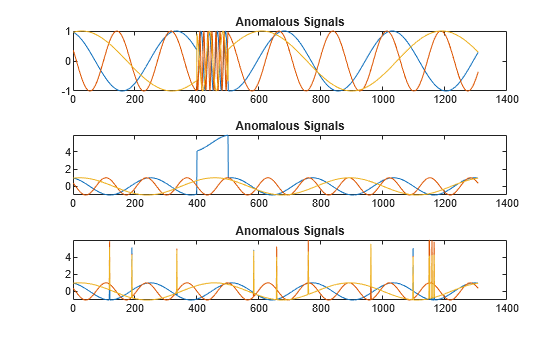
sineWaveAbnormal contains three signals, all of the same length. Each signal in the set has one or more anomalies.
All channels of the first signal have an abrupt change in frequency that lasts for a finite time.
The second signal has a finite-duration amplitude change in one of its channels.
The third signal has spikes at random times in all channels.
Create Detector
Use the timeSeriesLofAD detector to create a robust random cut forest detector with 3 channels and using "kdtree" and "cityblock" as the Search method / Distance metric pair.
detector_tslof = timeSeriesLofAD(3,SearchMethod="kdtree",Distance="cityblock")
detector_tslof =
  TimeSeriesLOFDetector with properties:

          NumNeighbors: []
              Distance: "cityblock"
            BucketSize: 50
             CacheSize: 1000
                   Cov: []
              Exponent: []
           IncludeTies: 0
          SearchMethod: "kdtree"
           NumChannels: 3
             IsTrained: 0
          WindowLength: 10
        TrainingStride: 1
       DetectionStride: 10
             Threshold: []
       ThresholdMethod: "kSigma"
    ThresholdParameter: 3
     ThresholdFunction: []
         Normalization: "zscore"
     FeatureExtraction: 1
Train Detector
Train the detector using the normal data.
detector_tslof = train(detector_tslof,sineWaveNormal);
View the threshold that train computes and saves within detector_tslof. This computed value is influenced by random factors, such as which subsets of the data are used for training, and can change somewhat for different training sessions and different machines.
thresh = detector_tslof.Threshold
thresh =
1.2772
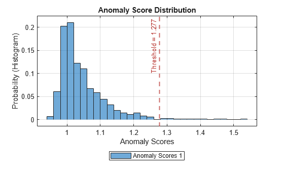
Plot Anomaly Scores
Plot the histogram of the anomaly scores for the normal data. Each score is calculated over a single detection window. The threshold, plotted as a vertical line, does not always completely bound the scores.
plotHistogram(detector_tslof,sineWaveNormal);
Use Detector to Identify Anomalies
Use the detect function to determine the anomaly scores for the anomalous data. Then, plot the anomaly scores of the normal and anomalous data together.
results = detect(detector_tslof, sineWaveAbnormal);
results is a cell array that contains three tables, one table for each signal. Each cell table contains three variables: WindowLabel, WindowAnomalyScore, and WindowStartIndices.
View the contents of the five rows between 10 and 15 of the third table.
results_table3 = results{3};
results_t3_rows10to15 = results_table3(10:15,:)results_t3_rows10to15=6×3 table
Labels AnomalyScores StartIndices
______ _____________ ____________
false 0.98275 91
false 1.0275 101
true 34.426 111
false 0.9937 121
false 1.0497 131
false 1.0424 141
The results indicate an anomaly in the third window of this set. The anomaly score is significantly higher than the scores for the other windows..
Plot Anomaly Score Distributions
Plot a histogram that shows the anomaly scores for both sets of data together, along with the threshold, for comparison.
plotHistogram(detector_tslof,sineWaveNormal,sineWaveAbnormal)
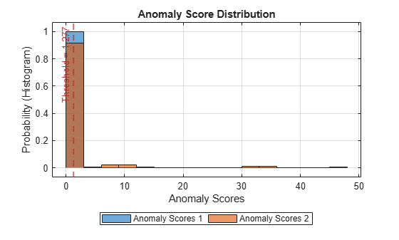
The histogram uses different colors for the normal (Data 1) and anomalous (Data 2) data. Both types of data appear to the left of the threshold. To the right of threshold, Data 2 is prevalent.
Plot Detected Anomalies
Plot the detected anomalies of the third abnormal signal set.
plot(detector_tslof,sineWaveAbnormal{3})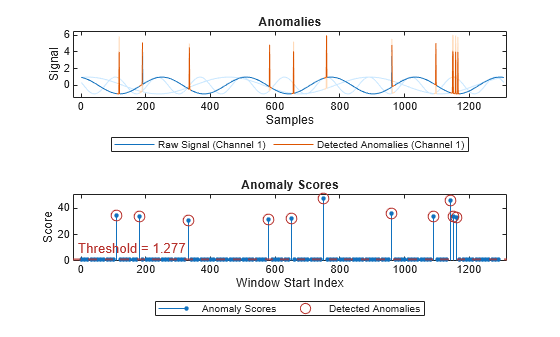
The top plot shows an overlay of red where the anomalies occur. The bottom plot shows how effective the threshold is at dividing the normal from the abnormal scores for Signal set 3.
Input Arguments
Name-Value Arguments
Output Arguments
Version History
Introduced in R2026a
See Also
train | detect | plot | plotHistogram | updateDetector