FPGA-Based Monopulse Technique: Algorithm Design
This example shows the first half part of a workflow to develop a monopulse technique where the signal is downconverted using digital downconversion (DDC). The model in this example is suitable for implementation on FPGA. This example focuses on the design of monopulse technique to estimate the azimuth and elevation of an object.
The second part of the example, FPGA-Based Monopulse Technique: Code Generation, shows how to generate HDL code from the implementation model and verify that the generated HDL code produces the correct results compared to the behavioral model. The entire algorithm is designed using fixed-point data types.
The example shows how to design an FPGA-ready monopulse technique to match a corresponding behavioral model in Simulink® using the Phased Array System Toolbox™, DSP HDL Toolbox™, and Fixed-Point Designer™. To verify the implementation model, the example compares the simulation output of the implementation model with the output of the behavioral model.
The Phased Array System Toolbox provides the floating-point behavioral model for the monopulse technique as a phased.MonopulseFeed System object™. DSP HDL Toolbox provides the FIR filter essential for the downconversion filtering.
Fixed-Point Designer provides data types and tools for developing fixed-point and single-precision algorithms to optimize performance on embedded hardware. Bit-true simulations can be performed to observe the impact of limited range and precision without implementing the design on hardware.
Monopulse is a technique where the received echoes from different elements of an antenna are used to estimate the direction of arrival (DOA) of a signal. This direction helps estimate the location of an object. The example uses DSP HDL Toolbox and Fixed-Point Designer to design the algorithm. This technique uses four beams to measure the angular position of the target. All the four beams are generated simultaneously and the difference of azimuth and elevation is achieved in a single pulse, hence, the name monopulse.
Designing the Subsystem
The algorithm is implemented by using Simulink® blocks that support HDL code generation. The model assumes that the signal is received from the 4-element uniform rectangular array (URA), so, the model has 4 sinusoids as inputs. Assuming a 4-element URA, the model is comprised of 4 receive channels from each of the elements of the URA. Once the signals are converted to the digital domain, DDC blocks ensure that the frequency of the received signal is lowered to reduce the sample rate for processing. The block diagram shows the subsystem which consists of the following modules.
Multi-Channel Input Signal
Digital Down-Conversion
Monopulse Sum and Difference Channels
modelname = 'SimulinkDDCMonopulseHDLWorkflowExample';
open_system(modelname);
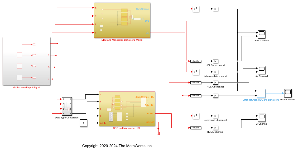
The Simulink model has two branches. The top branch is the behavioral floating-point model of the monopulse technique and digital downconversion algorithm and the bottom branch is the functionally equivalent fixed-point version using blocks that support HDL code generation. Apart from plotting the output of both branches to compare the two, the difference, or error, between sum channel of both the outputs has also been calculated and plotted.
The output of the behavioral model has a delay ( ) block. This delay is needed because the implementation algorithm uses 220 delays to enable pipelining which creates latency that needs to be accounted for. This latency is necessary to time-align the output between the behavioral model and the implementation model.
Digital DownConversion (DDC)
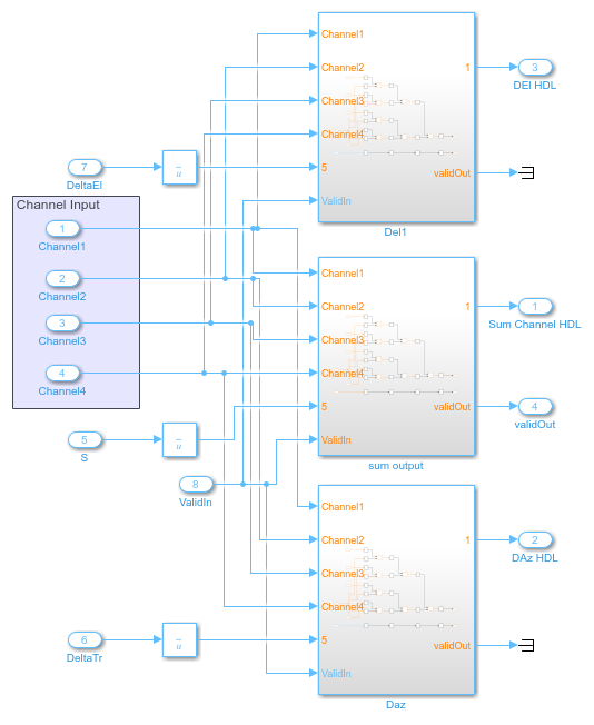
The DDC and Monopulse HDL subsystem shows how the received signal sampled at 80 MHz and nearly 15 MHz carrier frequency is downconverted to baseband via the DDC and then passed to the monopulse sum and difference subsystem. A DDC module is a combination of a numerically controlled oscillator (NCO) and a set of low-pass filters. The NCO block provides the signal to mix and demodulate the incoming signal.
open_system([modelname '/DDC and Monopulse HDL']);
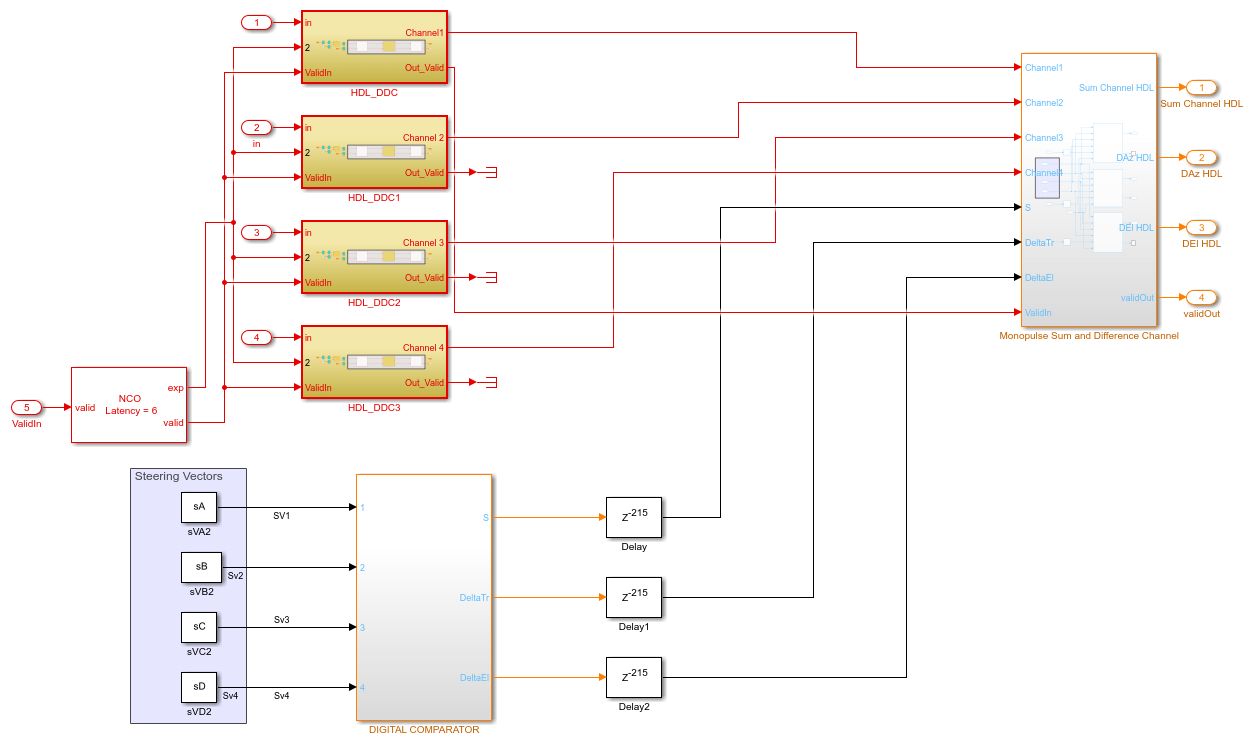
The delay of 215 ms at the sum and difference output of the steering vectors in the implementation subsystem compensates for the delay of the downconversion chain.
A DDC also contains a set of lowpass filters as shown in the figure. Once mixed, the lowpass filtering of the mixed signal is required to eliminate the high frequency components. This example uses a cascaded filter chain for lowpass filtering. The NCO generates the high-accuracy sinusoid for the mixer. The NCO block has a latency of 6 cycles. This signal is mixed with the incoming signal and is converted from a higher frequency to a relatively lower frequency as it progresses through the filter stages.
open_system([modelname '/DDC and Monopulse HDL/HDL_DDC']);
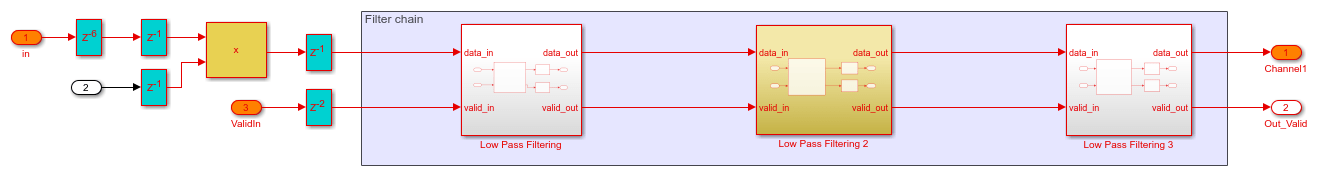
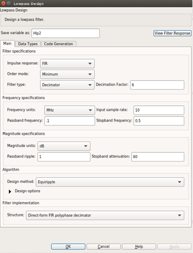
In this example, the incoming signal has a carrier frequency of 15 MHz and is sampled at 80 MHz. The downconversion process brings the sampled signal down to a few kHz. The coefficients for the lowpass FIR filters are designed using filterBuilder. The coefficient values must be chosen to satisfy the required passband criteria.
Once generated, the coefficients are used to configure the FIR Filter block.
Monopulse Sum and Difference Channels
The monopulse algorithm must also generate a steering vector for different elements. The steering vectors have been generated for an incident angle of azimuth 30 degrees and elevation 20 degrees. The steering vectors are passed to the digital comparator to provide the desired sum and difference channel outputs. The downconverted signal is then multiplied by the conjugate of these vectors as shown in the figure. By processing the sum and difference channels, the DOA of the received signal can be found. The digital comparator that compares the steering vectors for the different elements of the antenna array is shown.
open_system([modelname '/DDC and Monopulse HDL/DIGITAL COMPARATOR']);
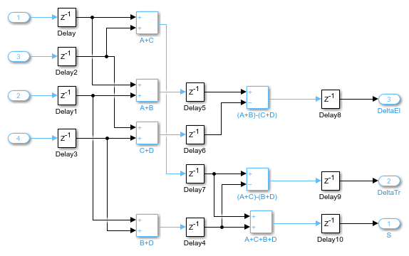
In the figure, the digital comparator takes the steering vectors and computes the sum and difference of the different steering vectors sVA, sVB, sVC and sVD respectively. You can also calculate the steering vectors by using the phased.SteeringVector System object or you can generate them using method similar to the one shown in the FPGA-Based Beamforming in Simulink: Algorithm Design. Once the sum and difference of various steering vectors corresponding to each element of the array has been done, the calculation of sum and difference channels for corresponding azimuth and elevation angles are performed. From the Sum and Difference Monopulse subsystem, 3 signals are obtained, namely the sum, the azimuth difference, and the elevation difference. The entire arithmetic is performed in fixed-point data types. Open the monopulse sum and difference channel subsystem by using this command.
open_system([modelname '/DDC and Monopulse HDL/Monopulse Sum and Difference Channel']);
Comparing Results of Implementation Model to Behavioral Model
To compare results of the implementation model to the behavioral model, run the model created to display the results. You can run the Simulink model by clicking the Play button or calling the sim command on the MATLAB® command line. Use Scope blocks to compare the output frames.
sim(modelname);

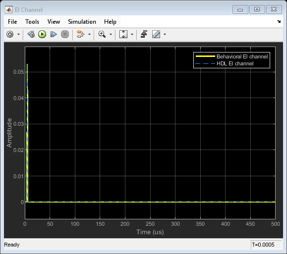
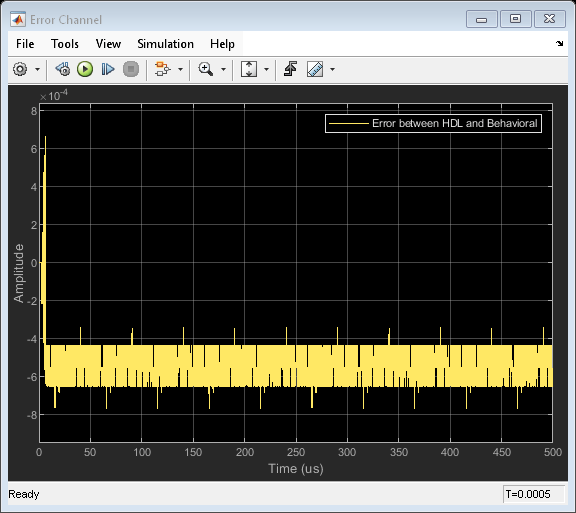
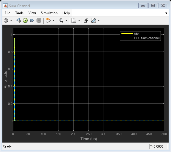
The plots show the output from sum and difference channels. These channels can be fed to an estimator to indicate the angle/direction of the object.
Summary
This example demonstrates how to design an FPGA-ready algorithm, automatically generate HDL code, and verify the HDL code in Simulink. The example illustrates the design of a Simulink model for a DDC and monopulse feed system, and verifies the results with an equivalent behavioral model from the Phased Array System Toolbox as the golden reference. Apart from the behavioral model, the example demonstrates how to create a subsystem for implementation using Simulink blocks that support HDL code generation. It also compared the output of the implementation model to the output of the corresponding behavioral model to verify that the two algorithms are functionally equivalent.
Once the implementation algorithm is functionally verified to be equivalent to golden reference, HDL Coder™ can be used for Simulink to HDL code generation and HDL Verifier™ can be used to Generate Cosimulation Model (HDL Coder) test bench.
The second part of this two-part series shows how to generate HDL code from the implementation model and verify that the generated HDL code produces the same results as the floating-point behavioral model as well as the fixed-point implementation model.