離散化された最適軌跡 (問題ベース)

R2026b

この例では、問題ベースのアプローチを使用して、離散化された最適軌跡問題を解く方法を示します。軌跡の重力は一定とし、印加される力には限度があり、空気抵抗は考慮しません。この解法プロセスは、固定期間 $T$ の間の最適な軌跡を求め、その解を使用して最適な $T$ 、つまりコストを最小限にする時間を見つけます。この例では、次に、空気抵抗を導入する方法を示し、最後に、オブジェクトが燃料を消費する際の可変質量の影響を導入する方法を示します。

最適化変数を使用して ODE のパラメーターを当てはめるの例のような離散化されていない最適化と比較して、離散化された最適化は常微分方程式 (ODE) を解く場合正確ではありません。しかし、離散化された最適化は、シミュレーションまたは常微分方程式の最適化の説明にあるとおり、可変ステップ ODE ソルバーに含まれるノイズの影響を受けません。また、離散化された最適化の方がカスタマイズしやすくなることがあり、モデル化も簡単です。最後に、離散化された最適化では、最適化プロセスで自動微分を活用できます。問題ベースの最適化における自動微分の効果を参照してください。

問題の説明

問題は、制御されたジェット機を使用して、時間 $0$ における位置 $p_{0}$ から時間 $T$ における位置 $p_{F}$ までオブジェクトを移動することです。位置はベクトル $p (t)$ 、速度はベクトル $v (t)$ 、印加された加速度はベクトル $a (t)$ で表します。連続時間では、重力を含めた運動方程式は次のようになります。

$\frac{d p}{d t} = v (t)$

$\frac{d v}{d t} = a (t) + g * [0, 0, - 1]$ .

ジェット機は加速度 $a (t)$ を印加します。結果として得られる加速度には重力の項が追加されます。

ジェット機が印加できる最大加速度は $A_{m a x} = 25$ です。

時間を離散化して問題を解きます。時間をサイズ $t = T / N$ で $N$ 個に等分割します。タイムステップ $i$ における位置はベクトル $p (i)$ 、速度はベクトル $v (i)$ 、印加された加速度はベクトル $a (i)$ となります。ODE モデルをかなり正確に表現する、一連の方程式を作成できます。近似運動方程式は次のようになります。

$v (i) = v (i - 1) + t (a (i - 1) + g), i = 1 . . . N$

$p (i) = p (i - 1) + t (\frac{v (i - 1) + v (i)}{2}), i = 1 . . . N .$

前述の方程式では、2 点 (台形則) 近似を使用して速度を積分し、1 点 (オイラー) 近似を使用して加速度を積分します。加速度 $a (i)$ が時間間隔の中心 $i$ に印加されるとみなした場合、積分法が加速度の中点則となります。積分法全体で得られる方程式は簡単なもので、ステップ $i$ における位置および速度は、ステップ $i - 1$ における位置、速度、および加速度のみに依存しています。この方程式は、空気抵抗を考慮するように変更するのも容易です。

境界条件は、 $p (0) = p_{0}$ 、 $p (N) = p_{F}$ 、および $v (0) = v (N) = [0, 0, 0]$ です。初期位置および最終位置は次のように設定します。

p0 = [0 0 0];
pF = [5 10 3];

MATLAB® のインデックスは 0 ではなく 1 から開始します。インデックス付けを容易にするために、区間数を $N - 1$ と指定し、位置と速度のインデックスを、 $0$ から $N$ ではなく、 $1$ から $N$ とします。このインデックス付けにより、加速度のインデックスは $1$ から $N - 1$ となります。

ジェット機を使用して、時間 $t$ の間に力 $a$ を発生させるのにかかるコストは、 $‖ a ‖ t$ です。総コストは、加速度と $t$ の積のノルムの和です。

$C o s t = \sum_{i = 1}^{N - 1} ‖ a (i) ‖ t .$

このコストを最適化変数の線形コストに変換するには、変数 $s (i)$ と、関連する 2 次錐制約を作成します。

$\begin{array}{l} C o s t = \sum_{i = 1}^{N - 1} s (i) t \\ ‖ a (i) ‖ \leq s (i) . \end{array}$

すべてのタイムステップについて、加速度のノルムが定数 Amax によって制限される追加制約を課します。

$‖ a (i) ‖ \leq A m a x .$

これらの制約も 2 次錐制約です。制約が線形または 2 次錐制約であり、目的関数が線形であるため、solve は coneprog ソルバーを呼び出して問題を解きます。coneprog ソルバーは非常に効率的です。次のセクションで確認するように、coneprog は十数回の反復で解を見つけます。一方で、fmincon は、可変質量を導入するためにモデルを拡張のセクションで変更した問題を解くために数千回の反復を実行します。

この例の最後の補助関数 setupproblem1 は、固定の時間 T の最適化問題を作成します。このコードでは、運動方程式を問題の制約として組み込んでいます。この関数には空気抵抗の引数が含まれています。空気抵抗を考慮するモデルの場合は、air = true と設定してください。空気抵抗の定義については、空気抵抗の導入のセクションを参照してください。

印加された加速度 $a$ が、この問題のメインの最適化変数となります。Vanderbei [1] が提案するように、この問題では速度 v と位置 p を最適化変数としてとる必要はありません。運動方程式と印加された加速度 $a$ の値から、それらの値を導き出すことができます。N ステップの場合、 $a$ の次元は N – 1 行 3 列となります。また、この問題には、線形目的関数を許可する最適化変数として、ベクトル変数 s が含まれています。

T = 20 について問題を解く

時間 $T = 20$ の軌跡問題を作成し、解きます。

[trajprob,p] = setupproblem1(20);

この問題の既定のソルバーは何でしょうか。

defaultsolver = solvers(trajprob)

defaultsolver = 
"coneprog"

coneprog ソルバーのオプションを設定して、問題を解きます。この問題では数値の厳密さが求められるため、信頼性を確保するために、最適性の許容誤差は 1e-9 に設定します。

opts = optimoptions(defaultsolver,Display="none",OptimalityTolerance=1e-9);
[sol,fval,eflag,output] = solve(trajprob,Options=opts)

sol = struct with fields:
    a: [49×3 double]
    s: [49×1 double]

fval = 
192.2812

eflag = 
    OptimalSolution

output = struct with fields:
           iterations: 11
    primalfeasibility: 4.4805e-10
      dualfeasibility: 1.9307e-09
           dualitygap: 3.3531e-11
            algorithm: 'interior-point'
         linearsolver: 'augmented'
              message: 'Optimal solution found.'
               solver: 'coneprog'

補助関数 plottrajandaccel を呼び出して、軌跡および加速度のノルムをプロットします。

N = 50;
plottrajandaccel(sol,p,p0,pF)

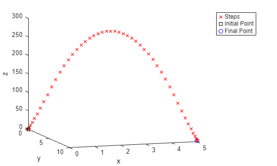
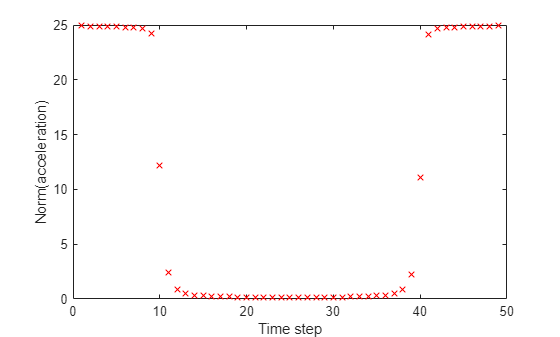
3-D plot of optimal trajectory from initial point to final point, showing an arc reaching height z = 270

Plot of norm of acceleration versus time step showing bang-bang behavior: maximal (25) at beginning and end, near zero in the middle

加速度は、期間の開始時点と終了時点でほぼ最大、中間時点でほぼゼロになります。このように、加速度が最大か 0 のいずれかになるような解を「バンバン」と呼びます。

最小コストの特定

時間 $T$ をいくつにすればコストが最小になるでしょうか。 $T = 1$ など時間が短すぎる場合、問題は実行不可能であり、したがって解はありません。

myprob = setupproblem1(1);
opts.Display = "final"; % To see the solution status
[solm,fvalm,eflagm,outputm] = solve(myprob,Options=opts);

Solving problem using coneprog.
Problem is infeasible.

時間を 1.5 にすると問題が実行可能になります。

myprob = setupproblem1(1.5);
[solm,fvalm,eflagm,outputm] = solve(myprob,Options=opts);

Solving problem using coneprog.
Optimal solution found.

補助関数 tomin は、時間 T の問題を設定してから、solve を呼び出して解となるコストを計算します。tomin 上で fminbnd を呼び出し、区間 $1.5 \leq T \leq 10$ における最適な時間 (できる限り低いコスト) を特定します。

[Tmin,Fmin] = fminbnd(@(T)tomin(T,false),1.5,10)

Tmin = 
1.9517

Fmin = 
24.6095

最適時間 Tmin の軌跡を求めます。

[minprob,p] = setupproblem1(Tmin);
sol = solve(minprob,Options=opts);

Solving problem using coneprog.
Optimal solution found.

最小となる軌跡と加速度をプロットします。

plottrajandaccel(sol,p,p0,pF)

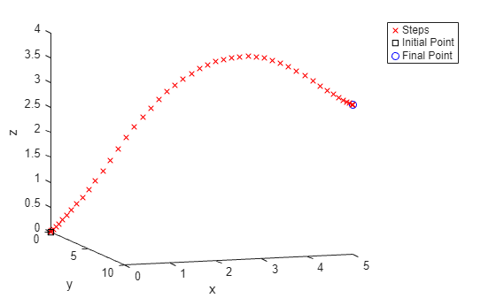
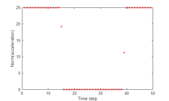
3-D plot of minimal-cost trajectory from initial point to final point, showing a lower arc reaching height z = 3.5

Plot of norm of acceleration versus time step showing nearly ideal bang-bang behavior: maximal (25) at beginning and end, exactly zero in the middle

最小となる解はほぼ「バンバン」解であり、加速度は 2 つの値を除くすべての値で最大かゼロのいずれかとなります。

最小とならない軌跡のプロット

さまざまな時間の軌跡をプロットします。

figure
hold on
options = optimoptions("coneprog",Display="none",OptimalityTolerance=1e-9);
g = [0 0 -9.81];
for i = 1:10
    T = 2*i;
    t = T/N;
    prob = setupproblem1(T);
    sol = solve(prob,Options=options);
    asol = sol.a;
    vsol = cumsum([[0 0 0];t*(asol+repmat(g,size(asol,1),1))]);
    N = size(vsol,1);
    np = 2:N;
    n0 = 1:(N-1);
    psol = cumsum([p0;t*(vsol(np,:) + vsol(n0,:))/2]);
plot3(psol(:,1),psol(:,2),psol(:,3),"rx",Color=[256-25*i 20*i 25*i]/256)
end
view([18 -10])
xlabel("x")
ylabel("y")
zlabel("z")
legend("T = 2","T = 4","T = 6","T = 8","T = 10","T = 12","T = 14","T = 16","T = 18","T = 20")
hold off

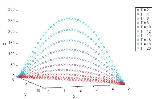
3-D plot of trajectories for T = 2 through T = 20, showing increasingly higher arcs as travel time increases

最も短い時間 (2) の軌跡は、このスケールではほぼ一直線となっています。時間が長くなるほど直線から大きくずれており、 $T = 20$ のパスは 300 付近の高さに達しています。

空気抵抗の導入

モデルのダイナミクスを変更して、空気抵抗を導入します。線形空気抵抗により、時間 $t$ 後に速度が係数 $\exp (- t)$ だけ変化します。運動方程式は次のようになります。

$v (i) = v (i - 1) \exp (- t) + t (a (i - 1) + g)$

$\begin{array}{l} p (i) = p (i - 1) + t (\frac{v (i - 1) + v (i)}{2}) \\ = p (i - 1) + t (\frac{1 + \exp (- t)}{2}) v (i - 1) + t^{2} \frac{a (i - 1) + g}{2} . \end{array}$

air = true の場合の関数 setupproblem1(T,air) の問題の定式化には、速度定数を定義する行および位置定数を定義する行の両方に exp(-t) の係数があります。

vcons(2:N,:) = v(2:N,:) == v(1:(N-1),:)*exp(-t) + t*(a(1:(N-1),:) + repmat(g,N-1,1));
pcons(2:N,:) = p(2:N,:) == p(1:(N-1),:) + t*(1+exp(-t))/2*v(1:(N-1),:) + t^2/2*(a(1:(N-1),:) + repmat(g,N-1,1));

空気抵抗を含む問題に対する最適な時間を求めます。

[Tmin2,Fmin2] = fminbnd(@(T)tomin(T,true),1.5,10)

Tmin2 = 
1.9399

Fmin2 = 
28.7967

最適な時間は、空気抵抗がない問題の時間よりわずかに小さいだけ (1.95 ではなく 1.94) ですが、コスト Fmin は約 17% 上昇します (24.6 ではなく 28.8)。

compartable = table([Tmin;Tmin2],[Fmin;Fmin2],VariableNames=["Time" "Cost"],RowNames=["Original" "Air Resistance"])

compartable = 2×2 table
    1.9517    24.6095
    1.9399    28.7967

空気抵抗を含む場合の最適解の軌跡および加速度をプロットします。

[minprob,p] = setupproblem1(Tmin2,true);
sol = solve(minprob,Options=opts);

Solving problem using coneprog.
Optimal solution found.

plottrajandaccel(sol,p,p0,pF)

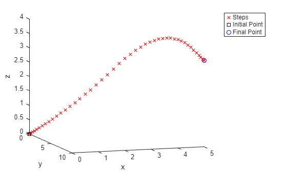
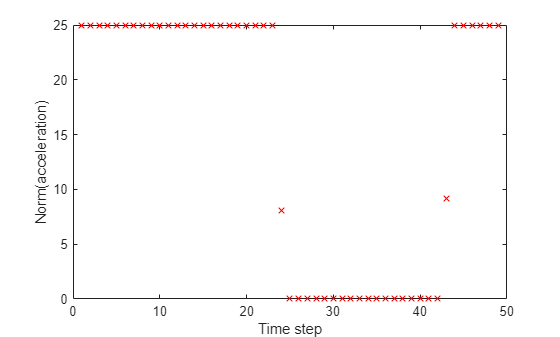
3-D plot of optimal trajectory with air resistance, similar arc shape reaching height z = 3.3

Plot of norm of acceleration versus time step with air resistance: maximal at beginning and end with zero-acceleration interval shifted to a later time

空気抵抗があると、ゼロ加速度の時間が後ろのタイムステップに移動し、短縮されます。ただし、解はほぼ「バンバン」のままです。

可変質量を導入するためにモデルを拡張

ジェット機は質量を放出することで動作します。ジェット機が動作する際に質量が減少する影響を含める場合、運動方程式は 2 次錐問題のフレームワークに当てはまらなくなります。問題を数値的に解くのが難しくなり、求解時間が長くなったり、解の精度が低下したりします。

モデルを変更して、印加される力 $F (t)$ と質量 $m (t)$ を含めます。正味加速度は以下です。

$a (t) = F (t) / m (t) + g [0, 0, - 1]$ .

質量の変化率は以下です。

$\frac{d m}{d t} = - r ‖ F (t) ‖,$

ここで、 $r$ は定数です。

$m (0) = 2$ 、 $r = 1 / 1000$ 、最大力が $F_{m a x} = 50$ と仮定します。これらの仮定から、時間 0 における印加された最大加速度は $F_{m a x} / m (0) = 25$ となり、前のモデルと同じ最大加速度であることがわかります。

関数 setupproblemfuel1 は、これらの方程式とパラメーターに基づいて問題を作成します。可変質量モデルのこのインスタンスには空気抵抗を導入しません。

[trajprob,p] = setupproblemfuel1(20);

結果として得られる問題の既定のソルバーは何でしょうか。

defaultsolver = solvers(trajprob)

defaultsolver = 
"fmincon"

fmincon ソルバーは初期点を必要とします。T = 20 でランダムな初期点を試してみてください。

rng default
y0 = randn(49,3);
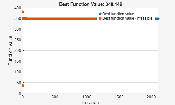
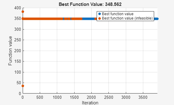
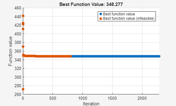
x0.F = y0;

ソルバーが進行状況に応じてプロットを生成し、既定よりも多くの関数評価と反復を行えるようにソルバーのオプションを指定します。StepTolerance を既定の 1e-10 から 1e-11 に減らして精度を上げてみてください。

opts = optimoptions(defaultsolver,Display="none",PlotFcn="optimplotfvalconstr",...
    MaxFunctionEvaluations=1e5,MaxIterations=1e4,StepTolerance=1e-11);

ソルバーを呼び出します。

[sol,fval,eflag,output] = solve(trajprob,x0,Options=opts)

Optimization plot showing best function value converging to 348.149 over 2000 iterations, with initial infeasible values

sol = struct with fields:
    F: [49×3 double]

fval = 
348.1493

eflag = 
    StepSizeBelowTolerance

output = struct with fields:
              iterations: 2114
               funcCount: 7024
         constrviolation: 4.2188e-13
                stepsize: 3.8563e-11
               algorithm: 'interior-point'
           firstorderopt: 0.0060
            cgiterations: 59677
                 message: 'Local minimum possible. Constraints satisfied.↵↵fmincon stopped because the size of the current step is less than↵the value of the step size tolerance and constraints are ↵satisfied to within the value of the constraint tolerance.↵↵<stopping criteria details>↵↵Optimization stopped because the relative changes in all elements of x are↵less than options.StepTolerance = 1.000000e-11, and the relative maximum constraint↵violation, 2.225061e-16, is less than options.ConstraintTolerance = 1.000000e-06.'
            bestfeasible: [1×1 struct]
     objectivederivative: 'reverse-AD'
    constraintderivative: 'reverse-AD'
                  solver: 'fmincon'

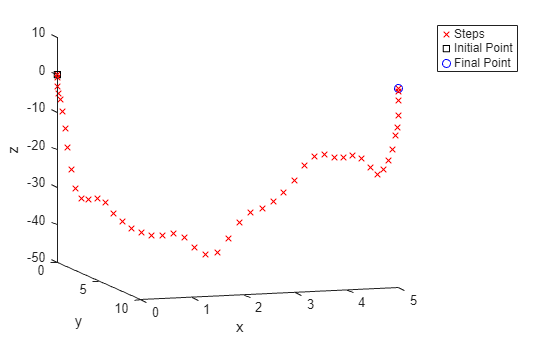
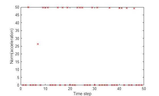
軌跡と加速度をプロットします。関数 plottrajandaccel は解の構造体の a フィールドにこの値を使用するため、まず F フィールドから a フィールドに解をコピーします。

sol.a = sol.F;
plottrajandaccel(sol,p,p0,pF)

3-D plot of trajectory with variable mass model showing erratic path dropping below z = -50

Plot of norm of acceleration versus time step showing oscillatory ringing behavior between 0 and 50

可変加速度のコストを追加して解を平滑化

印加される力は基本的に「バンバン」ですが、この力には振動運動があります。Vanderbei [1] はこのタイプの動作を「リンギング」と呼びます。リンギングをなくすには、振動加速度のコストを追加し、再度解きます。補助関数 setupproblemfuel2 には、目的関数の追加項 t*1e-4*sum(diff(fnorm).^2 が含まれており、加速度のノルム変位にペナルティを設定します。

 % Add cost for acceleration changes
 trajectoryprob.Objective = sum(fnorm)*t + t*1e-4*sum(diff(fnorm).^2);

問題を再度解きます。

[trajprob,p] = setupproblemfuel2(20);
[sol,fval,eflag,output] = solve(trajprob,x0,Options=opts)

Optimization plot showing best function value converging to 348.562 over 3500 iterations

sol = struct with fields:
    F: [49×3 double]

fval = 
348.5616

eflag = 
    StepSizeBelowTolerance

output = struct with fields:
              iterations: 3922
               funcCount: 8024
         constrviolation: 2.4034e-12
                stepsize: 8.9591e-11
               algorithm: 'interior-point'
           firstorderopt: 0.1031
            cgiterations: 45717
                 message: 'Local minimum possible. Constraints satisfied.↵↵fmincon stopped because the size of the current step is less than↵the value of the step size tolerance and constraints are ↵satisfied to within the value of the constraint tolerance.↵↵<stopping criteria details>↵↵Optimization stopped because the relative changes in all elements of x are↵less than options.StepTolerance = 1.000000e-11, and the relative maximum constraint↵violation, 1.267582e-15, is less than options.ConstraintTolerance = 1.000000e-06.'
            bestfeasible: [1×1 struct]
     objectivederivative: 'reverse-AD'
    constraintderivative: 'reverse-AD'
                  solver: 'fmincon'

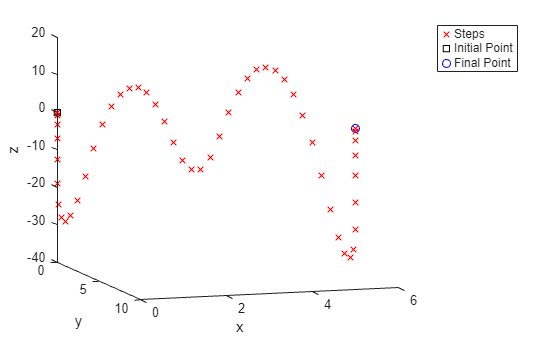
sol.F データを使用して軌跡と加速度をプロットします。

sol.a = sol.F;
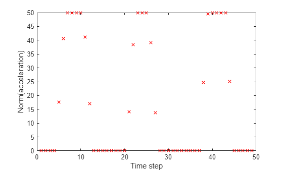
plottrajandaccel(sol,p,p0,pF)

3-D plot of trajectory with smoothing penalty showing irregular path with z values between -40 and 20

Plot of norm of acceleration versus time step still showing oscillatory behavior between 0 and 50, with multiple intervals of zero force

より適切な初期点の指定

ほとんどのリンギングはなくなりましたが、解にはまだ力がゼロの区間が複数あります。

別の初期点を指定することで、より満足のいく解を得られる可能性があります。ソルバーの中間時点の加速度を小さくするには、インデックス 10 から 40 の場合は 0 に等しい初期点を、インデックス 1 から 9 および 41 から 49 の場合は 20 に等しい初期点を指定します。初期点にランダムノイズを追加します。

rng default
y0 = 20*ones(49,3);
y0(10:40,:) = 0;
y0 = y0 + randn(size(y0));
x0.F = y0;

この新しい点から始めて問題を解きます。

[sol,fval,eflag,output] = solve(trajprob,x0,Options=opts)

Optimization plot showing best function value converging to 348.277 over 2200 iterations with decreasing infeasible values

sol = struct with fields:
    F: [49×3 double]

fval = 
348.2770

eflag = 
    StepSizeBelowTolerance

output = struct with fields:
              iterations: 2289
               funcCount: 8050
         constrviolation: 5.2673e-12
                stepsize: 3.7699e-11
               algorithm: 'interior-point'
           firstorderopt: 0.1509
            cgiterations: 59337
                 message: 'Local minimum possible. Constraints satisfied.↵↵fmincon stopped because the size of the current step is less than↵the value of the step size tolerance and constraints are ↵satisfied to within the value of the constraint tolerance.↵↵<stopping criteria details>↵↵Optimization stopped because the relative changes in all elements of x are↵less than options.StepTolerance = 1.000000e-11, and the relative maximum constraint↵violation, 4.536371e-15, is less than options.ConstraintTolerance = 1.000000e-06.'
            bestfeasible: [1×1 struct]
     objectivederivative: 'reverse-AD'
    constraintderivative: 'reverse-AD'
                  solver: 'fmincon'

軌跡と加速度をプロットします。

sol.a = sol.F;
plottrajandaccel(sol,p,p0,pF)

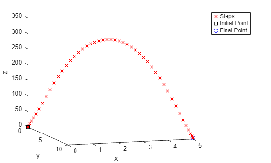
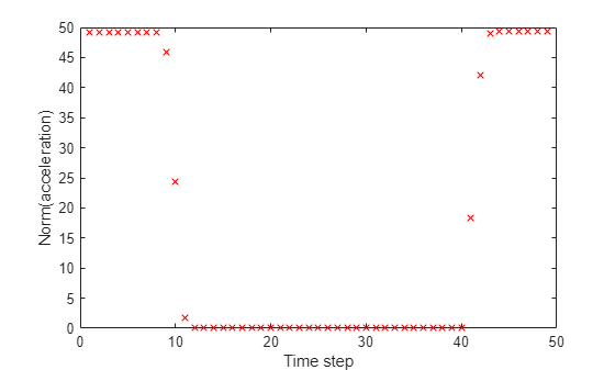
3-D plot of satisfactory trajectory showing smooth arc reaching height z = 300, similar to the original solution

Plot of norm of acceleration versus time step showing nearly bang-bang behavior with one interval of zero applied force

満足のいく解が得られたようです。これは基本的に、印加された加速度がゼロの区間が 1 つだけの「バンバン」の加速度です。

オブジェクトの移動が終わったとき、最初の 2 からどれだけの質量が残っているでしょうか。

T = 20;
N = 50;
t = T/N;
fnorm = zeros(N-1,1);
r = 1/1000;
for i = 1:length(fnorm)
    fnorm(i) = norm(sol.F(i,:));
end
m = 2 - r*t*sum(fnorm)

m = 
1.6518

このように質量が減少した場合、印加された最大加速度はどのくらいになるでしょうか。

Fmax = 50;
Fmax/m

ans = 
30.2700

モデルに可変質量の影響が導入されている場合、軌跡の間の印加された最大加速度は 25 から 30 に変わります。

空気抵抗と可変質量の導入

モデルに再度空気抵抗を導入します。この場合、補助関数 setupproblemfuel2 が fcn2optimexpr を使用して補助関数 airResistance を呼び出し、空気抵抗を考慮した速度を評価します。別の関数を使用して for ループをコーディングし、fcn2optimexpr を使用してその関数を呼び出すと、より効率的な問題が作成されます。詳細については、静的解析のための for ループの作成と最適化式の静的解析を参照してください。

[trajprob2,p] = setupproblemfuel2(20,true);

空気抵抗を導入した先ほどのモデルの結果に基づき、力がゼロの初期区間を、10 から 40 ではなく、15 から 45 に設定します。

rng default
y0 = 20*ones(49,3);
y0(15:45,:) = 0;
y0 = y0 + randn(size(y0));
x0.F = y0;

問題を解きます。

[sol2,fval2,eflag2,output2] = solve(trajprob2,x0,Options=opts)

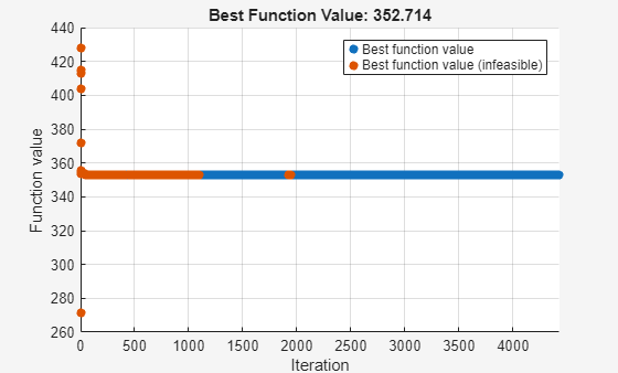
Optimization plot showing best function value converging to 352.714 over 4000 iterations

sol2 = struct with fields:
    F: [49×3 double]

fval2 = 
352.7138

eflag2 = 
    StepSizeBelowTolerance

output2 = struct with fields:
              iterations: 4434
               funcCount: 8676
         constrviolation: 9.4591e-13
                stepsize: 5.6003e-11
               algorithm: 'interior-point'
           firstorderopt: 0.2388
            cgiterations: 66173
                 message: 'Local minimum possible. Constraints satisfied.↵↵fmincon stopped because the size of the current step is less than↵the value of the step size tolerance and constraints are ↵satisfied to within the value of the constraint tolerance.↵↵<stopping criteria details>↵↵Optimization stopped because the relative changes in all elements of x are↵less than options.StepTolerance = 1.000000e-11, and the relative maximum constraint↵violation, 6.606756e-15, is less than options.ConstraintTolerance = 1.000000e-06.'
            bestfeasible: [1×1 struct]
     objectivederivative: 'reverse-AD'
    constraintderivative: 'reverse-AD'
                  solver: 'fmincon'

sol2.a = sol2.F;
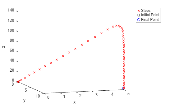
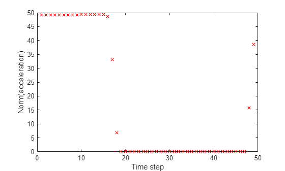
plottrajandaccel(sol2,p,p0,pF)

3-D plot of trajectory for longer time horizon showing arc reaching height z = 120 with steep descent near the final point

Plot of norm of acceleration versus time step showing bang-bang behavior with zero force in the middle portion

残った燃料の質量はどのくらいになるでしょうか。

for i = 1:length(fnorm)
    fnorm(i) = norm(sol2.F(i,:));
end
m2 = 2 - r*t*sum(fnorm)

m2 = 
1.6474

このように質量が減少した場合、印加された最大加速度はどのくらいになるでしょうか。

Fmax/m2

ans = 
30.3517

空気抵抗を導入しても燃料消費量は大きく変わりません。この軌跡では空気抵抗を利用してオブジェクトを減速させているようで、オブジェクトは移動の最後の部分では減速にあまり燃料を使用していません。空気抵抗のある軌跡の最大の高さは 130 未満ですが、空気抵抗のない軌跡の最大の高さは約 300 であることに注意してください。現在のパラメーターでは、空気抵抗によって軌跡に有意差が出ますが、燃料消費量には有意差が出ません。

参考文献

[1] Vanderbei, R. J. "Case Studies in Trajectory Optimization: Trains, Planes, and Other Pastimes." Optimization and Engineering 2, 215–243 (2001). https://vanderbei.princeton.edu/tex/trajopt/trajopt.pdf から入手可能。

補助関数

次のコードは、setupproblem1 補助関数を作成します。

function [trajectoryprob,p] = setupproblem1(T,air)
    if nargin == 1
        air = false;
    end
    N = 50; % Number of steps
    g = [0 0 -9.81]; % Gravitational acceleration
    p0 = [0 0 0]; % Initial position
    pF = [5 10 3]; % Final position
    Amax = 25; % Maximum applied acceleration
    t = T/N; % Time steps
    a = optimvar("a",N-1,3,LowerBound=-Amax,UpperBound=Amax);
    v = optimexpr(N,3);
    trajectoryprob = optimproblem;
    s = optimvar("s",N-1,LowerBound=0,UpperBound=3*Amax); % Norm of applied acceleration
    trajectoryprob.Objective = sum(s)*t;
    scons = optimconstr(N-1);
    for i = 1:(N-1)
        scons(i) = norm(a(i,:)) <= s(i); % Cone constraint
    end
    acons = optimconstr(N-1);
    for i = 1:(N-1)
        acons(i) = norm(a(i,:)) <= Amax; % Cone constraint
    end
    np = 2:N;
    n0 = 1:(N-1);
    v0 = [0 0 0];
    if air
        v(1, :) = v0;
        for i = 2:N
            v(i,:) = v(i-1,:)*exp(-t) + t*(a(i-1,:) + g); % Linear in optimization variables 
        end
    else
        gbig = repmat(g,size(a,1),1);
        v = cumsum([v0; t*(a + gbig)]); % v is the sum of applied accelerations and gravity
    end
    p = cumsum([p0;t*(v(np,:) + v(n0,:))/2]); % Independent of "air"
    endcons = v(N,:) == [0 0 0]; % Land with zero velocity
    pcons2 = p(N,:) == pF; % End at the specified position
    trajectoryprob.Constraints.acons = acons;
    trajectoryprob.Constraints.scons = scons;
    trajectoryprob.Constraints.endcons = endcons;
    trajectoryprob.Constraints.pcons2 = pcons2;
end

次のコードは、plottrajandaccel 補助関数を作成します。

function plottrajandaccel(sol,p,p0,pF)
figure
psol = evaluate(p, sol);
plot3(psol(:,1),psol(:,2),psol(:,3),"rx")
hold on
plot3(p0(1),p0(2),p0(3),"ks")
plot3(pF(1),pF(2),pF(3),"bo")
hold off
view([18 -10])
xlabel("x")
ylabel("y")
zlabel("z")
legend("Steps","Initial Point","Final Point")
figure
asolm = sol.a;
nasolm = sqrt(sum(asolm.^2,2));
plot(nasolm,"rx")
xlabel("Time step")
ylabel("Norm(acceleration)")
end

次のコードは、tomin 補助関数を作成します。

function F = tomin(T,air) % F = cost of optimal trajectory over time T
    if nargin == 1
        air = false;
    end
    problem = setupproblem1(T,air);
    opts = optimoptions("coneprog",Display="none",OptimalityTolerance=1e-9);
    [~,F] = solve(problem,"Options",opts);
end

次のコードは、setupproblemfuel1 補助関数を作成します。

function [trajectoryprob,p] = setupproblemfuel1(T,air)
    r = 1/1000;
    if nargin == 1
        air = false;
    end
    N = 50; % Number of steps
    g = [0 0 -9.81]; % Gravitational acceleration
    p0 = [0 0 0]; % Initial position
    pF = [5 10 3]; % Final position
    Fmax = 50; % Maximum force
    t = T/N; % Time steps
    F = optimvar("F",N-1,3,LowerBound=-Fmax,UpperBound=Fmax); % Force
    v = optimexpr(N,3);
    fnorm = sqrt(sum(F(1:N-1,:).^2,2)); % Norm at each step
    m = 2 - r*t*cumsum(fnorm); % Mass diminishes proportional to norm of F
    trajectoryprob = optimproblem;
    trajectoryprob.Objective = sum(fnorm)*t;
    Fcons = fnorm <= Fmax;
    v0 = [0 0 0];
    if air
        v = fcn2optimexpr(@airResistance,v,v0,N,t,F,m,g);
    else
        gbig = repmat(g,size(F,1),1);
        mbig = repmat(m,1,3);
        v = cumsum([v0; t*(F./mbig + gbig)]);
    end
    np = 2:N;
    n0 = 1:(N-1);
    p = cumsum([p0;t*(v(np,:) + v(n0,:))/2]); % Independent of "air"
    endcons = v(N,:) == [0 0 0];
    pcons2 = p(N,:) == pF;
    trajectoryprob.Constraints.Fcons = Fcons;
    trajectoryprob.Constraints.endcons = endcons;
    trajectoryprob.Constraints.pcons2 = pcons2;
end

次のコードは、setupproblemfuel2 補助関数を作成します。

function [trajectoryprob,p] = setupproblemfuel2(T,air)
    r = 1/1000;
    if nargin == 1
        air = false;
    end
    N = 50;
    g = [0 0 -9.81];
    p0 = [0 0 0];
    pF = [5 10 3];
    Fmax = 50;
    t = T/N;
    F = optimvar("F",N-1,3,LowerBound=-Fmax,UpperBound=Fmax);
    v = optimexpr(N,3);
    fnorm = sqrt(sum(F(1:N-1,:).^2,2));
    m = 2 - r*t*cumsum(fnorm);
    trajectoryprob = optimproblem;
    % Add cost for acceleration changes
    trajectoryprob.Objective = sum(fnorm)*t + t*1e-4*sum(diff(fnorm).^2);
    Fcons = fnorm <= Fmax;
    v0 = [0 0 0];
    if air
        v = fcn2optimexpr(@airResistance,v,v0,N,t,F,m,g);
    else
        gbig = repmat(g,size(F,1),1);
        mbig = repmat(m,1,3);
        v = cumsum([v0; t*(F./mbig + gbig)]); % v is the sum of applied accelerations and gravity
    end
    np = 2:N;
    n0 = 1:(N-1);
    p = cumsum([p0;t*(v(np,:) + v(n0,:))/2]); % Independent of "air"
    endcons = v(N,:) == [0 0 0]; % Land with zero velocity
    pcons2 = p(N,:) == pF; % End at the specified position
    trajectoryprob.Constraints.Fcons = Fcons;
    trajectoryprob.Constraints.endcons = endcons;
    trajectoryprob.Constraints.pcons2 = pcons2;
end

次のコードは、setupproblemfuel1 と setupproblemfuel2 で使用される補助関数 airResistance を作成します。

function v = airResistance(v,v0,N,t,F,m,g)
v(1,:) = v0;
for i = 2:N
    v(i,:) = v(i-1,:)*exp(-t) + t*(F(i-1,:)/m(i-1) + g);
end
end

参考

coneprog | solve