バナナ関数の最小化

この例では、Rosenbrock の "バナナ関数" を最小化する方法を示します。

$$f(x)=100(x(2)-x(1{)}^2{)}^2+(1-x(1){)}^2.$$

$$f(x)$$ は、原点付近の曲率のため、バナナ関数と呼ばれます。この問題を解こうとするとほとんどの方法で収束が遅くなるため、最適化の例の中で悪名高いものとなっています。

$$f(x)$$ には点 $$x=[1,1]$$ に一意な最小値があり、$$f(x)=0$$ です。この例では、点 $$x0=[-1.9,2]$$ を開始点として $$f(x)$$ を最小化する方法をいくつか示します。

導関数を使用しない最適化

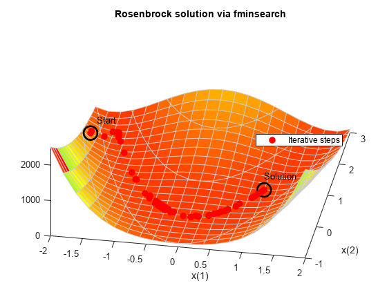
関数 fminsearch によって制約のない問題の最小値を見つけます。ここでは目的関数の導関数を推定しないアルゴリズムが使用されます。代わりに、幾何学的探索法が使用されます (fminsearch アルゴリズムを参照)。

fminsearch を使用してバナナ関数を最小化します。一連の反復をレポートする出力関数を含めます。

fun = @(x)(100*(x(2) - x(1)^2)^2 + (1 - x(1))^2);
options = optimset('OutputFcn',@bananaout,'Display','off');
x0 = [-1.9,2];
[x,fval,eflag,output] = fminsearch(fun,x0,options);
title 'Rosenbrock solution via fminsearch'

Fcount = output.funcCount;
disp(['Number of function evaluations for fminsearch was ',num2str(Fcount)])

Number of function evaluations for fminsearch was 210

disp(['Number of solver iterations for fminsearch was ',num2str(output.iterations)])

Number of solver iterations for fminsearch was 114

推定された導関数を使用した最適化

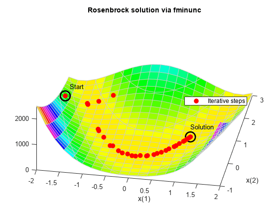
関数 fminunc によって制約のない問題の最小値を見つけます。ここでは導関数に基づくアルゴリズムが使用されます。このアルゴリズムは、目的関数の 1 次導関数だけでなく 2 次導関数の行列も推定しようと試みます。通常、fminunc は fminsearch よりも効率的です。

fminunc を使用してバナナ関数を最小化します。

options = optimoptions('fminunc','Display','off',...
    'OutputFcn',@bananaout,'Algorithm','quasi-newton');
[x,fval,eflag,output] = fminunc(fun,x0,options);
title 'Rosenbrock solution via fminunc'

Fcount = output.funcCount;
disp(['Number of function evaluations for fminunc was ',num2str(Fcount)])

Number of function evaluations for fminunc was 150

disp(['Number of solver iterations for fminunc was ',num2str(output.iterations)])

Number of solver iterations for fminunc was 34

最急降下法を使用した最適化

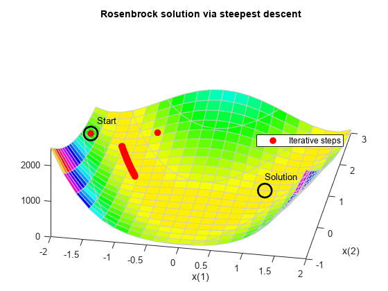
最急降下アルゴリズムを使用してバナナ関数を最小化しようとすると、問題の曲率が高いために解法プロセスが非常に遅くなります。

最急降下アルゴリズムを使用する fminunc を実行するには、'quasi-newton' アルゴリズムの HessUpdate 非表示オプションを値 'steepdesc' に設定します。ソルバーで解を求めるのに時間がかかるため、関数評価の最大回数を既定よりも大きな値に設定してください。この場合は、関数評価が 600 回実行された後でも解が求められません。

options = optimoptions(options,'HessUpdate','steepdesc',...
    'MaxFunctionEvaluations',600);
[x,fval,eflag,output] = fminunc(fun,x0,options);
title 'Rosenbrock solution via steepest descent'

Fcount = output.funcCount;
disp(['Number of function evaluations for steepest descent was ',...
    num2str(Fcount)])

Number of function evaluations for steepest descent was 600

disp(['Number of solver iterations for steepest descent was ',...
    num2str(output.iterations)])

Number of solver iterations for steepest descent was 45

解析勾配を使用した最適化

勾配を与えると、fminunc で最適化を解決する際に使用される関数評価が少なくなります。勾配を与える場合は、'quasi-newton' アルゴリズムに比べて高速になることが多く、メモリ使用量も少なくなる 'trust-region' アルゴリズムを使用できます。HessUpdate オプションと MaxFunctionEvaluations オプションを既定値にリセットします。

grad = @(x)[-400*(x(2) - x(1)^2)*x(1) - 2*(1 - x(1));
            200*(x(2) - x(1)^2)];
fungrad = @(x)deal(fun(x),grad(x));
options = resetoptions(options,{'HessUpdate','MaxFunctionEvaluations'});
options = optimoptions(options,'SpecifyObjectiveGradient',true,...
    'Algorithm','trust-region');
[x,fval,eflag,output] = fminunc(fungrad,x0,options);
title 'Rosenbrock solution via fminunc with gradient'

Fcount = output.funcCount;
disp(['Number of function evaluations for fminunc with gradient was ',...
    num2str(Fcount)])

Number of function evaluations for fminunc with gradient was 32

disp(['Number of solver iterations for fminunc with gradient was ',...
    num2str(output.iterations)])

Number of solver iterations for fminunc with gradient was 31

解析的ヘッシアンを使用した最適化

ヘッシアン (2 次導関数の行列) を与えると、fminunc で最適化を解決する際に使用される関数評価をさらに少なくすることができます。この問題では、ヘッシアンを使用してもしなくても結果は同じです。

hess = @(x)[1200*x(1)^2 - 400*x(2) + 2, -400*x(1);
            -400*x(1), 200];
fungradhess = @(x)deal(fun(x),grad(x),hess(x));
options.HessianFcn = 'objective';
[x,fval,eflag,output] = fminunc(fungradhess,x0,options);
title 'Rosenbrock solution via fminunc with Hessian'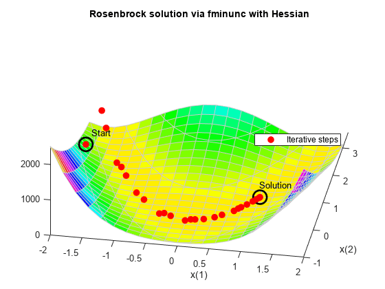

Fcount = output.funcCount;
disp(['Number of function evaluations for fminunc with gradient and Hessian was ',...
    num2str(Fcount)])

Number of function evaluations for fminunc with gradient and Hessian was 32

disp(['Number of solver iterations for fminunc with gradient and Hessian was ',num2str(output.iterations)])

Number of solver iterations for fminunc with gradient and Hessian was 31

最小二乗ソルバーを使用した最適化

非線形二乗和に推奨されるソルバーは、lsqnonlin です。このソルバーは、この特別なクラスの問題において勾配を使用しない fminunc よりもさらに効率的です。lsqnonlin を使用する場合は、目的関数を二乗和として記述しないでください。代わりに、lsqnonlin によって内部的に二乗和される基礎となるベクトルを記述してください。

options = optimoptions('lsqnonlin','Display','off','OutputFcn',@bananaout);
vfun = @(x)[10*(x(2) - x(1)^2),1 - x(1)];
[x,resnorm,residual,eflag,output] = lsqnonlin(vfun,x0,[],[],options);
title 'Rosenbrock solution via lsqnonlin'

Fcount = output.funcCount;
disp(['Number of function evaluations for lsqnonlin was ',...
    num2str(Fcount)])

Number of function evaluations for lsqnonlin was 87

disp(['Number of solver iterations for lsqnonlin was ',num2str(output.iterations)])

Number of solver iterations for lsqnonlin was 28

最小二乗ソルバーおよびヤコビアンを使用した最適化

fminunc で勾配を使用して最小化する場合と同様に、lsqnonlin で導関数情報を使用すると、関数評価の回数を減らすことができます。非線形目的関数ベクトルのヤコビアンを与えて、最適化を再実行します。

jac = @(x)[-20*x(1),10;
           -1,0];
vfunjac = @(x)deal(vfun(x),jac(x));
options.SpecifyObjectiveGradient = true;
[x,resnorm,residual,eflag,output] = lsqnonlin(vfunjac,x0,[],[],options);
title 'Rosenbrock solution via lsqnonlin with Jacobian'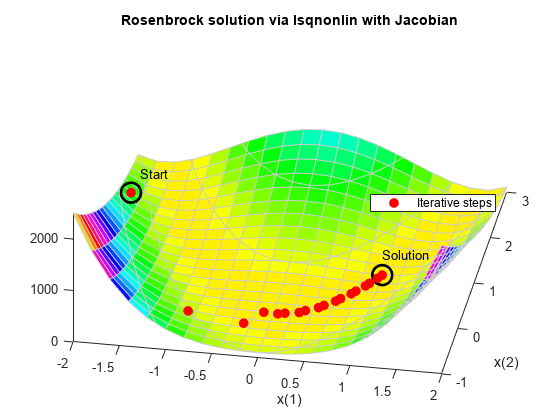

Fcount = output.funcCount;
disp(['Number of function evaluations for lsqnonlin with Jacobian was ',...
    num2str(Fcount)])

Number of function evaluations for lsqnonlin with Jacobian was 29

disp(['Number of solver iterations for lsqnonlin with Jacobian was ',...
    num2str(output.iterations)])

Number of solver iterations for lsqnonlin with Jacobian was 28

Copyright 2006–2020 The MathWorks, Inc.

関連するトピック

• [最適化] ライブ エディター タスクまたはソルバーを使用した制約付き非線形問題
• Symbolic Math Toolbox を使用した勾配とヘッシアンの計算

×

例を開く

この例の変更されたバージョンがあります。編集された方の例を開きますか?

いいえ、変更されたバージョンを上書きします。 はい