このページの内容は最新ではありません。最新版の英語を参照するには、ここをクリックします。

最大存在量分類を使用したハイパースペクトル イメージ解析

この例では、最大存在量分類 (MAC) を実行して、ハイパースペクトル イメージ内のさまざまな領域を識別する方法を示します。存在量マップは、ハイパースペクトル イメージ全体でエンドメンバー分布の特徴を表すものです。イメージ内の各ピクセルは、"ピュア ピクセル" の場合や "ミクセル" の場合があります。各ピクセルについて取得した存在量値のセットは、そのピクセルに存在する各エンドメンバーの割合を表しています。この例では、ピクセルごとの最大存在量値を見つけ、それを関連するエンドメンバー クラスに割り当てることでハイパースペクトル イメージ内のピクセルを分類します。

この例では、Image Processing Toolbox™ Hyperspectral Imaging Library が必要となります。Image Processing Toolbox Hyperspectral Imaging Library はアドオン エクスプローラーからインストールできます。アドオンのインストールの詳細については、アドオンの取得と管理を参照してください。Image Processing Toolbox Hyperspectral Imaging Library は MATLAB® Online™ および MATLAB® Mobile™ ではサポートされないため、デスクトップの MATLAB® が必要となります。

この例では、パヴィア大学のデータセットのデータ サンプルをテスト データとして使用します。このテスト データには、次のグラウンド トゥルース クラスを表す 9 つのエンドメンバーが格納されています。アスファルト、牧草地、砂利、樹木、塗装済み金属シート、露出土壌、瀝青、セルフ ブロック レンガ、影。

データの読み込みと可視化

テスト データを含む .mat ファイルをワークスペースに読み込みます。.mat ファイルには、ハイパースペクトル データ キューブを表す配列 paviaU、およびハイパースペクトル データから取得した 9 つのエンドメンバー シグネチャを表す行列 signatures が格納されています。データ キューブには、430 nm ～ 860 nm までの範囲の波長を持つ 103 個のスペクトル バンドがあります。幾何学的分解能は 1.3 メートル、各バンド イメージの空間分解能は 610 x 340 です。

load('paviaU.mat');
img = paviaU;
sig = signatures;

波長範囲をスペクトル バンドの数で均等間隔に分けることで、各スペクトル バンドの中心波長を計算します。

wavelengthRange = [430 860];
numBands = 103;
wavelength = linspace(wavelengthRange(1),wavelengthRange(2),numBands);

ハイパースペクトル データ キューブと中心波長を使用して hypercube オブジェクトを作成します。次に、ハイパースペクトル データから RGB イメージを推定します。RGB 出力のコントラストを改善するために、ContrastStretching パラメーター値を true に設定します。RGB イメージを可視化します。

hcube = hypercube(img,wavelength);
rgbImg = colorize(hcube,'Method','RGB','ContrastStretching',true);
figure
imshow(rgbImg)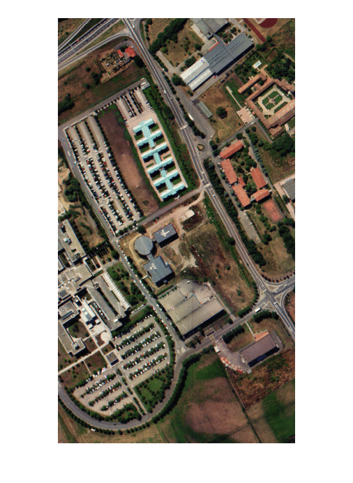

テスト データには、9 つのグラウンド トゥルース クラスのエンドメンバー シグネチャが格納されています。sig の各列には、1 つのグラウンド トゥルース クラスのエンドメンバー シグネチャが格納されています。各エンドメンバーのクラス名と sig の対応する列を一覧表示する table を作成します。

num = 1:size(sig,2);
endmemberCol = num2str(num');
classNames = {'Asphalt';'Meadows';'Gravel';'Trees';'Painted metal sheets';'Bare soil';...
              'Bitumen';'Self blocking bricks';'Shadows'};
table(endmemberCol,classNames,'VariableName',{'Column of sig';'Endmember Class Name'})

ans=9×2 table
    Column of sig      Endmember Class Name  
    _____________    ________________________

          1          {'Asphalt'             }
          2          {'Meadows'             }
          3          {'Gravel'              }
          4          {'Trees'               }
          5          {'Painted metal sheets'}
          6          {'Bare soil'           }
          7          {'Bitumen'             }
          8          {'Self blocking bricks'}
          9          {'Shadows'             }

エンドメンバーのシグネチャをプロットします。

figure
plot(sig)
xlabel('Band Number')
ylabel('Data Values')
ylim([400 2700])
title('Endmember Signatures')
legend(classNames,'Location','NorthWest')

存在量マップの推定

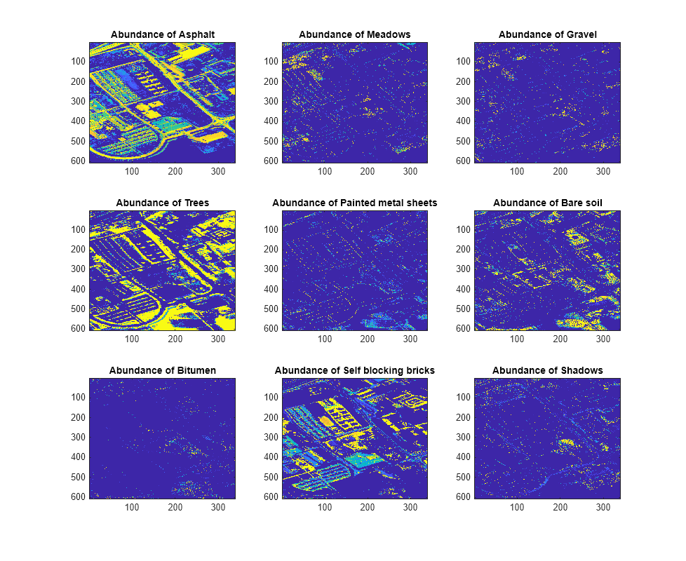
関数 estimateAbundanceLS を使用してエンドメンバーの存在量マップを作成し、完全制約付き最小二乗 (FCLS) 法を選択します。関数は、空間次元を入力データとして使用し、3 次元配列として存在量マップを出力します。各チャネルは、シグネチャの対応する列からのエンドメンバーの存在量マップです。この例では、入力データの空間次元は 610 × 340 で、エンドメンバーの数は 9 です。したがって、出力存在量マップのサイズは 610 x 340 x 9 となります。

abundanceMap = estimateAbundanceLS(hcube,sig,'Method','fcls');

存在量マップを表示します。

fig = figure('Position',[0 0 1100 900]);
n = ceil(sqrt(size(abundanceMap,3)));
for cnt = 1:size(abundanceMap,3)
    subplot(n,n,cnt)
    imagesc(abundanceMap(:,:,cnt))
    title(['Abundance of ' classNames{cnt}])
    hold on
end
hold off

最大存在量分類の実行

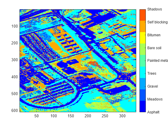
各ピクセルの最大存在量値のチャネル数を見つけます。各ピクセルについて返されるチャネル数は、そのピクセルの最大存在量値に関連するエンドメンバー シグネチャを含む sig 内の列に対応しています。最大存在量値で分類したピクセルの色分けイメージを表示します。

[~,matchIdx] = max(abundanceMap,[],3);
figure
imagesc(matchIdx)
colormap(jet(numel(classNames)))
colorbar('TickLabels',classNames)

分類された領域をセグメント化し、ハイパースペクトル データ キューブから推定された RGB イメージにそれぞれを重ね合わせます。

segmentImg = zeros(size(matchIdx));
overlayImg = zeros(size(abundanceMap,1),size(abundanceMap,2),3,size(abundanceMap,3));
for i = 1:size(abundanceMap,3)
    segmentImg(matchIdx==i) = 1;
    overlayImg(:,:,:,i) = imoverlay(rgbImg,segmentImg);
    segmentImg = zeros(size(matchIdx));
end

クラス名とともに、分類および重ね合わせたハイパースペクトル イメージの領域を表示します。イメージから、アスファルト、樹木、露出土壌、セルフ ブロック レンガの領域が正確に分類されていることが分かります。

figure('Position',[0 0 1100 900]);
n = ceil(sqrt(size(abundanceMap,3)));
for cnt = 1:size(abundanceMap,3)
    subplot(n,n,cnt);
    imagesc(uint8(overlayImg(:,:,:,cnt)));
    title(['Regions Classified as ' classNames{cnt}])
    hold on
end
hold off

参考

estimateAbundanceLS | hypercube | colorize

関連するトピック

• ハイパースペクトル イメージ処理入門