Create and Display 3-D Mask of DICOM-RT Contour Data
This example shows how to create a binary mask of ROI data stored in the metadata of a DICOM-RT structure set file, and display the mask as an overlay on the underlying image data.
A DICOM-RT structure set is a DICOM Information Object Definition (IOD) specific to radiotherapy. The metadata of a DICOM-RT structure set file includes contour data for regions of interest (ROIs) relevant to radiation treatment planning. The metadata specifies ROI data as boundary coordinates, with separate contours for each slice. This example converts the contours defining a brain tumor ROI into a single 3-D binary mask. You can display the mask as an overlay by using the volshow function or the Volume Viewer app.
Load Image Data and Metadata
This example uses a modified subset of data from the BraTS data set [1] [2]. The data includes a brain MRI scan, as well as ROI contour data for a tumor within the scan region.
Load the brain MRI image volume into the workspace. The image volume is stored in the MAT file vol_001.mat.
load(fullfile(toolboxdir("images"),"imdata", ...
    "BrainMRILabeled","images","vol_001.mat"));
Read the metadata from the DICOM-RT structure set file brainMRI_rt.dcm, attached to this example as a supporting file. The file contains contour data for the brain tumor ROI.
info = dicominfo("brainMRI_rt.dcm");Extract ROI Data from DICOM-RT Metadata
Create a dicomContours object containing the ROI contour data stored in the metadata structure info.
rtContours = dicomContours(info);
Display the ROI information as a table. Each element in the ContourData cell array specifies the xy-coordinates of the boundary points in one axial slice. The 'Brain Tumor' ROI consists of 56 closed planar contours.
rtContours.ROIs
ans=1×5 table
    Number         Name          ContourData    GeometricType       Color
    ______    _______________    ___________    _____________    ____________

      1       {'Brain Tumor'}    {56×1 cell}     {56×1 cell}     {3×1 double}
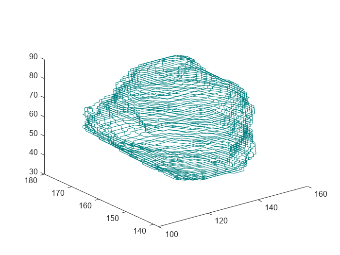
Plot the contours of the 'Brain Tumor' ROI by using the plotContours object function.
figure
plotContour(rtContours)
Create 3-D Binary Mask of ROI
Define the spatial referencing for the ROI by creating an imref3d object with the same number of slices and pixel size as the brain MRI image data. The pixel size is 1-by-1-by-1 mm, meaning that each pixel of the MRI image data corresponds to a section of the brain with length, width, and height of 1 mm each.
referenceInfo = imref3d(size(vol),1,1,1);
Create a 3-D logical mask of the 'Brain Tumor' ROI. This corresponds to the first ROI index in rtContours, so specify the ROIindex input as 1. Specify the imref3d object to define spatial information for the mask.
rtMask = createMask(rtContours,1,referenceInfo);
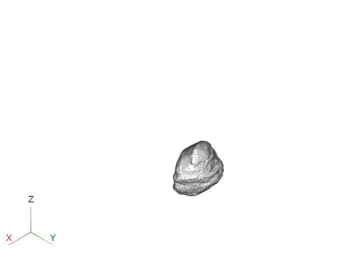
Display the mask by using the volshow function.
viewer = viewer3d(BackgroundColor="white",BackgroundGradient="off",CameraZoom=1.5);
maskDisp = volshow(rtMask,Parent=viewer);
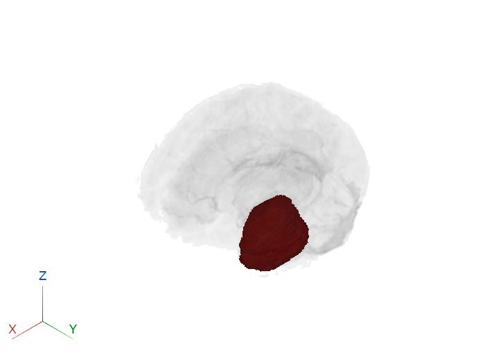
Display ROI Mask as Image Overlay Using volshow
Display the binary tumor mask as an overlay on the MRI image data by using the volshow function.
viewer = viewer3d(BackgroundColor="white",BackgroundGradient="off",CameraZoom=1.5);
volDisp = volshow(vol,OverlayData=rtMask,Parent=viewer, ...
    RenderingStyle="GradientOpacity",GradientOpacityValue=0.8, ...
    Alphamap=linspace(0,0.2,256),OverlayAlpha=0.8);
Display ROI Mask as Image Overlay Using Volume Viewer
You can also visualize the position of the ROI in the 3-D slice planes of the brain MRI image using the Volume Viewer app. Load the brain as an intensity volume and the tumor mask as a labeled volume into the Volume Viewer app by using the volumeViewer command.
volumeViewer(vol,double(rtMask));
To display the mask in the 3-D slice planes of the intensity volume, on the app toolstrip, select Slice Planes. Use the scroll bars in the three slice panes to change the position of the slice planes in the 3-D Volume window. For more details about viewing labeled volumes using the Volume Viewer app, see Explore 3-D Labeled Volumetric Data with Volume Viewer.

References
[1] Isensee, Fabian, Philipp Kickingereder, Wolfgang Wick, Martin Bendszus, and Klaus H. Maier-Hein. “Brain Tumor Segmentation and Radiomics Survival Prediction: Contribution to the BRATS 2017 Challenge.” In Brainlesion: Glioma, Multiple Sclerosis, Stroke and Traumatic Brain Injuries, edited by Alessandro Crimi, Spyridon Bakas, Hugo Kuijf, Bjoern Menze, and Mauricio Reyes, 10670:287–97. Cham: Springer International Publishing, 2018. https://doi.org/10.1007/978-3-319-75238-9_25.
[2] Medical Segmentation Decathlon. "Brain Tumours." Tasks. Accessed May 10, 2018. http://medicaldecathlon.com/.
The BraTS data set is provided by Medical Segmentation Decathlon under the CC-BY-SA 4.0 license. All warranties and representations are disclaimed. See the license for details. MathWorks® has modified the subset of data used in this example. This example uses the MRI and label data of one scan from the original data set. The MRI image data has been converted to a MAT file, and the tumor label data has been converted to a DICOM-RT structure set file.
See Also
dicomContours | createMask | plotContour | Volume Viewer