Reproduce Command Line or System Identification App Simulation Results in Simulink
Once you identify a model, you can simulate it at the command line, in the System Identification app, or in Simulink®. If you start with one simulation method, and migrate to a second method, you may find that the results do not precisely match. This mismatch does not mean that one of the simulations is implemented incorrectly. Each method uses a unique simulation algorithm, and yields results with small numeric differences.
Generally, command-line simulation functions such as compare and
sim,as well as the System Identification app, use
similar default settings and solvers. Simulink uses somewhat different default settings and a different solver. If you
want to validate your Simulink implementation against command-line or app simulation results, you must
ensure that your Simulink settings are consistent with your command-line or app simulation settings.
The following paragraphs list these settings in order of decreasing significance.
Initial Conditions
The most significant source of variation when trying to reproduce results is
usually the initial conditions. The initial conditions that you specify for
simulation in Simulink blocks must match the initial conditions used by
compare, sim, or the System
Identification app. You can determine the initial conditions returned in
the earlier simulations. Or, if you are simulating against measurement data, you can
estimate a new set of initial conditions that best match that data. Then, apply
those conditions to any simulation methods that you use. For more information on
estimating initial conditions, see Estimate Initial Conditions for Simulating Identified Models.
Once you have determined the initial conditions x0 to use for a
model m and a data set z, implement them in
your simulation tool.
For
compareorsim, usecompareOptionsorsimOptions.For Simulink, use the Idmodel, Nonlinear ARX Model, or Hammerstein-Wiener Model block, specifying
mfor the model andx0for the initial states. With Idmodel structures, you can specify initial states only foridssandidgreymodels. If your linear model is of any other type, convert it first toidss. See Simulate Identified Model in Simulink or the corresponding block reference pages.For the System Identification app, you cannot specify initial conditions other than zero. You can specify only the method of computing them.
Discretization of Continuous-Time Data
Simulink software assumes a first-order-hold interpolation on input data.
When using compare, sim, or the app, set
the InterSample property of your iddata
object to 'foh'.
Solvers for Continuous-Time Models
The compare command and the app simulate a continuous-time
model by first discretizing the model using c2d and then propagating the
difference equations. Simulink defaults to a variable-step true ODE solver. To better match the
difference-equation propagation, set the solver in Simulink to a fixed-step solver such as ode5.
Match Output of sim Command and Nonlinear ARX Model Block
Reproduce command-line sim results for an estimated nonlinear system in Simulink®. When you have an estimated system model, you can simulate it either with the command-line sim command or with Simulink. The two outputs do not match precisely unless you base both simulations on the same initial conditions. You can achieve this match by estimating the initial conditions in your MATLAB® model and applying both in the sim command and in your Simulink model.
Load the estimation data you are using to identify a nonlinear ARX model. Create an iddata data object from the data. Specify the sample time as 0.2 seconds.
load twotankdata
z = iddata(y,u,0.2);
Use the first 1000 data points to estimate a nonlinear ARX model mw1 with orders [5 1 3] and wavelet network nonlinearity.
z1 = z(1:1000);
mw1 = nlarx(z1,[5 1 3],idWaveletNetwork);
To initialize your simulated response consistently with the measured data, estimate an initial state vector x0 from the estimation data z1 using the findstates function. The third argument for findstates in this example, Inf, sets the prediction horizon to infinity in order to minimize the simulation error.
x0 = findstates(mw1,z1,Inf);
Simulate the model mw1 output using x0 and the first 50 seconds (250 samples) of input data.
opt = simOptions('InitialCondition',x0);
data_sim = sim(mw1,z1(1:251),opt);
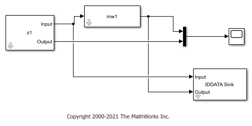
Now simulate the output of mw1 in Simulink using a Nonlinear ARX Model block, and specify the same initial conditions in the block. The Simulink model ex_idnlarx_block_match_sim is preconfigured to specify the estimation data, nonlinear ARX model, initial conditions x0, and a simulation time of 50 seconds.
Open the Simulink model.
model = 'ex_idnlarx_block_match_sim';
open_system(model);
Simulate the nonlinear ARX model output for 50 seconds.
sim(model);
The IDDATA Sink block outputs the simulated output, data, to the MATLAB workspace.
Plot and compare the simulated outputs you obtained using the sim command and Nonlinear ARX block.
figure
plot(data_sim.SamplingInstants,data_sim.OutputData,'b*',...
    data.SamplingInstants,data.OutputData,'-r')
xlabel('Time(sec)');
ylabel('Simulated output');
legend('Output of sim command','Output of Nonlinear ARX block','location','southeast')
title('Estimated Initial Conditions for Simulink')
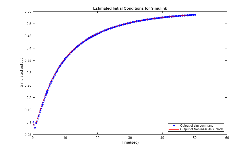
The simulated outputs are the same because you specified the same initial condition when using sim and the Nonlinear ARX Model block.
If you want to see what the comparison would look like without using the same initial conditions, you can rerun the Simulink version with no initial conditions set.
Nullify initial-condition vector x0, and simulate for 50 seconds as before. This null setting of x0 is equivalent to the Simulink initial conditions default.
x0 = [0;0;0;0;0;0;0;0];
sim(model);
Plot the difference between the command-line and Simulink methods for this case.
figure
plot(data_sim.SamplingInstants,data_sim.OutputData,'b*',...
    data.SamplingInstants,data.OutputData,'-r')
xlabel('Time(sec)');
ylabel('Simulated output');
legend('Output of sim command','Output of Nonlinear ARX block','location','southeast')
title('Default Initial Conditions for Simulink')
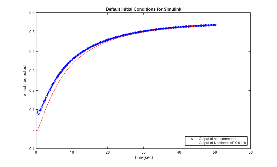
The Simulink version starts at a different point than the sim version, but the two versions eventually converge. The sensitivity to initial conditions is important for verifying reproducibility of the model, but is usually a transient effect.
Match Output of compare Command and Nonlinear ARX Model Block
In this example, you first use the compare command to match the simulated output of a nonlinear ARX model to measured data. You then reproduce the simulated output using a Nonlinear ARX Model block.
Load estimation data to estimate a nonlinear ARX model. Create an iddata object from the data. Specify the sample time as 0.2 seconds.
load twotankdata
z = iddata(y,u,0.2);
Use the first 1000 data points to estimate a nonlinear ARX model mw1 with orders [5 1 3] and wavelet network nonlinearity.
z1 = z(1:1000);
mw1 = nlarx(z1,[5 1 3],idWaveletNetwork);
Use the compare command to match the simulated response of mw1 to the measured output data in z1.
data_compare = compare(mw1,z1);
The compare function uses the first nx samples of the input-output data as past data, where nx is the largest regressor delay in the model. compare uses this past data to compute the initial states, and then simulates the model output for the remaining nx+1:end input data.
To reproduce this result in Simulink®, compute the initial state values used by compare, and specify the values in the Nonlinear ARX Model block. First compute the largest regressor delay in the model. Use this delay to compute the past data for initial condition estimation.
nx = max(getDelayInfo(mw1));
past_data = z1(1:nx);
Use data2state to get state values using the past data.
x0 = data2state(mw1,z1(1:nx));
Now simulate the output of mw1 in Simulink using a Nonlinear ARX Model block, and specify x0 as the initial conditions in the block. Use the remaining nx+1:end data for simulation.
zz = z1(nx+1:end);
zz.Tstart = 0;
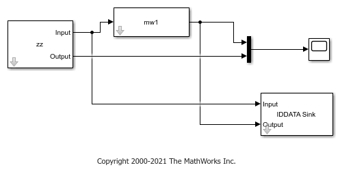
The Simulink model ex_idnlarx_block_match_compare is preconfigured to specify the estimation data, nonlinear ARX model, and initial conditions.
Open the Simulink model.
model = 'ex_idnlarx_block_match_compare';
open_system(model);
Simulate the nonlinear ARX model output for 200 seconds.
sim(model);
The IDDATA Sink block outputs the simulated output, data, to the MATLAB® workspace.
Compare the simulated outputs you obtained using the compare command and Nonlinear ARX block. To do so, plot the simulated outputs.
To compare the output of compare to the output of the Nonlinear ARX Model block, discard the first nx samples of data_compare.
data_compare = data_compare(nx+1:end);
data.Tstart=1;
plot(data_compare,data,'r--')
xlabel('Time(sec)');
legend show
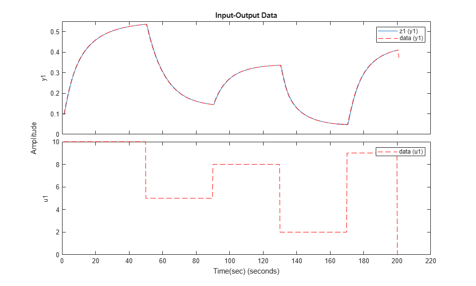
The simulated outputs are the same because you specified the same initial condition when using compare and the Nonlinear ARX Model block.
See Also
Nonlinear ARX Model | Hammerstein-Wiener Model | Nonlinear Grey-Box Model | compare | sim