メインコンテンツ

nlssinit

Initialize nonlinear state-space model using measured time-domain system data

Since R2026a

    Description

    nssInitialized = nlssinit(U,Y,nss) uses measured input and output data sets U and Y, and default training options, to train the state and output networks of the idNeuralStateSpace object nss. It estimates the weights and biases of the networks by numerically approximating the state derivatives and performing an open-loop training. The open-loop training minimizes the state-derivative prediction error for continuous-time models and the state-update prediction error for discrete-time models. This syntax returns the idNeuralStateSpace object nssInitialized with the trained state and output networks. You can use nssInitialized as the initial model when estimating neural state-space models using nlssest.

    nssInitialized = nlssinit(Data,nss) uses measured input and output data stored in Data, and the default training options, to train the state and output networks of nss.

    nssInitialized = nlssinit(___,Options) specifies custom training options, which use either the Adam, SGDM, RMSProp, or L-BFGS algorithm to train the networks.

    example

    nssInitialized = nlssinit(___,Name=Value) specifies name-value pair arguments after any of the input argument in the previous syntax. Use name-value pair arguments to specify whether you want to use the last experiment for validation, and the frequency for the validation plots.

    [nssInitialized,params] = nlssinit(___) returns model parameters corresponding to the final loss and minimal training loss. If UseLastExperimentForValidation is true, it also returns the model parameters corresponding to minimal validation loss.

    Examples

    collapse all

    This example demonstrates how to estimate a neural state-space model using both approximate open-loop and closed-loop training approaches. The example also compares the performance of the trained models on a validation data set.

    Load and Preprocess Data

    Load the two tank system data. The data consists of one input, u, and one output, y, signal.

    data = load("twotankdata.mat");
    u = data.u;
    y = data.y;

    Normalize the input and output data for better training performance.

    u = normalize(u);
    y = normalize(y);

    Split the data into training and validation sets and create iddata objects.

    zt = iddata(y(1:2000),u(1:2000),Ts=0.2);
    zv = iddata(y(2001:end),u(2001:end),Ts=0.2);

    To reproduce the results of this example, use a random generator seed.

    rng("default");

    Create Neural State-Space Model

    Create a discrete-time neural state-space model with one state and one input using idNeuralStateSpace.

    nx = 1;
    nu = 1;
    nss = idNeuralStateSpace(nx,NumInputs=nu,Ts=0.2);

    Define the structure of the state network to be a multi-layer perceptron (MLP) network with two hidden layers of 20 neurons each using createMLPNetwork.

    nss.StateNetwork = createMLPNetwork(nss,"state",LayerSizes=[20 20]);

    Specify Training Options

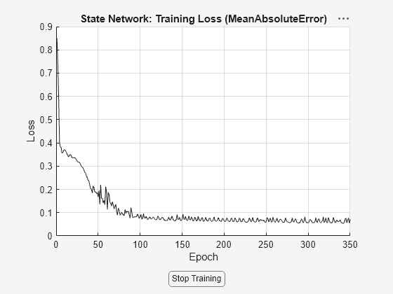
    Specify training options for the state network using nssTrainingOptions. Use the Adam algorithm, specify the maximum number of epochs as 350, and specify the window size as 128. For closed-loop training, the window size value decides the simulation horizon. For open-loop training, the prediction horizon is fixed to one.

    opt = nssTrainingOptions('adam');
    opt.MaxEpochs = 350;
    opt.WindowSize = 128;

    Estimate Neural State-Space Model

    Perform approximate open-loop training of the neural state-space model using nlssinit. Record the estimation time.

    tic
    sys1 = nlssinit(zt,nss,opt)
    Generating estimation report...done.
    
    sys1 =
    
    Discrete-time Neural ODE in 1 variables
         x(t+1) = f(x(t),u(t))
           y(t) = x(t) + e(t)
     
    f(.) network:
      Deep network with 2 fully connected, hidden layers
      Activation function: tanh
     
    Variables: x1
    Sample time: 0.2 seconds
     
    Status:                                           
    Estimated using NLSSINIT on time domain data "zt".
    Fit to estimation data: 87.18%                    
    FPE: 0.02567, MSE: 0.01539                        
    
    Model Properties
    
    t1 = toc
    t1 = 
    14.7177
    

    Estimate the model using closed-loop training approach using nlssest. Record the estimation time.

    tic
    sys2 = nlssest(zt,nss,opt)

    Figure Loss contains an axes object and another object of type uigridlayout. The axes object with title State Network: Training Loss (MeanAbsoluteError), xlabel Epoch, ylabel Loss contains an object of type animatedline.

    Generating estimation report...done.
    
    sys2 =
    
    Discrete-time Neural ODE in 1 variables
         x(t+1) = f(x(t),u(t))
           y(t) = x(t) + e(t)
     
    f(.) network:
      Deep network with 2 fully connected, hidden layers
      Activation function: tanh
     
    Variables: x1
    Sample time: 0.2 seconds
     
    Status:                                          
    Estimated using NLSSEST on time domain data "zt".
    Fit to estimation data: 88.33%                   
    FPE: 0.02127, MSE: 0.01275                       
    
    Model Properties
    
    t2 = toc
    t2 = 
    43.7440
    

    From the estimation times, you can see that open-loop training takes less time than the closed-loop training. The difference in estimation times between the training approaches becomes more obvious if you train the model with a large data set and turn off the plot, that is, specify the PlotLossFcn property of the training options object as false. For more details on the difference, see Training Neural State-Space Models.

    Compare Model Performance

    Compare the performance of both the trained models using the validation data set.

    compare(sys1,zv)
    compare(sys2,zv)

    MATLAB figure

    MATLAB figure

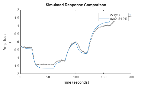
    As shown in this example, if the noise in the data is small or if the model exhibits a relatively low degree of nonlinearity, the model trained using approximate open-loop training approach can perform as good as the model trained using closed-loop training approach. So when given a data set, first use nlssinit to train the model as it is faster than closed-loop training. If the model performance is not good, you can use nlssest to perform closed-loop training by using this trained model as a starting point.

    Input Arguments

    collapse all

    Input data. Specify U as:

    • A timetable containing a variable for each input. The variable names of the timetable must match the input names of nss, and its row times must be duration objects. This timetable represents a single experiment. For more information, see timetable and duration.

    • A double matrix with one column for each input signal and one row for each time step. Use this option only if the system is discrete-time (that is nss.Ts is greater than zero). This matrix represents a single experiment.

    • A cell array of N experiments composed of timetables or double matrices. All the experiments must contain the same time points. In other words the time vector corresponding to all the observations must match.

    • An empty array, [], if nss has no inputs (that is size(nss,2) is zero).

    Output data. Specify Y as:

    • A timetable containing a variable for each output. The variable names of the timetable must match the output names of nss, and its row times must be duration objects. This timetable represents a single experiment. For more information, see timetable and duration.

    • A double matrix with one column for each output signal and one row for each time step. Use this option only if the system is discrete-time (that is nss.Ts is greater than zero). This matrix represents a single experiment.

    • A cell array of N experiments composed of timetables or double matrices. All the experiments must contain the same time points. In other words the time vector corresponding to all the observations must match.

    Note

    The first nx channels in Y must be state measurements (here, nx is the number of states specified in nss).

    Input and output data, specified as a timetable or iddata object. This argument allows you to specify the training data using a single input argument rather than separate U and Y arguments. Specify Data as one of the following:

    • An iddata object. If you have multiple experiments, create a multi-experiment iddata object. Use this option if all the input and output variables in an experiment share the time vector. For more information, see merge (iddata).

    • A timetable. The timetable must contain a variable for each of the input and output variables in nss. In the multi-experiment case, use a cell array of timetables. All the timetables in the cell array must use the same time vector.

    Neural state-space system, specified as an idNeuralStateSpace object.

    Training options, specified as an nssTrainingADAM, nssTrainingSGDM, nssTrainingRMSProp, or nssTrainingLBFGS object. Create the training options set object options using the nssTrainingOptions command. If nss contains a non-state output network (that is, if nss.OutputNetwork contains two networks), you can pick different training options for the state transition function network, nss.StateNetwork, and the nontrivial output function nss.OutputNetwork(2). Note that nss.OutputNetwork(1) does not contain any learnable parameters because it is always fixed to the identity function returning all the states as outputs.

    Name-Value Arguments

    collapse all

    Specify optional pairs of arguments as Name1=Value1,...,NameN=ValueN, where Name is the argument name and Value is the corresponding value. Name-value arguments must appear after other arguments, but the order of the pairs does not matter.

    Example: UseLastExperimentForValidation = true

    Option to use the last experiment for validation, specified as one of the following:

    • true — The last experiment is not used for training, but only to display a validation plot after a number of epochs specified by ValidationFrequency. This allows you to monitor the estimation performance during the training process. The last experiment can have a different duration than all the other experiments

    • false — All experiments are used for training, and no validation plot is displayed.

    Validation frequency, specified as a positive integer. This is the number of epochs after which the validation plot is updated with a new comparison (new predicted output against measured outputs).

    If you return additional model parameters (params) as an output, for every n number of epochs, where n is the ValidationFrequency, the software computes the validation loss. This validation loss corresponds to the loss at the nth epoch. In each epoch, the software computes the training loss. The software then compares all the training and validation losses and saves the lowest training loss, the lowest validation loss, and their corresponding model parameters.

    Output Arguments

    collapse all

    Initialized neural state-space system, returned as an idNeuralStateSpace object.

    Additional model parameters corresponding to final loss, minimal training loss, and minimal validation loss (if applicable), returned as a table with four columns.

    The first column displays the type of loss. If UseLastExperimentForValidation is true, this column displays "Final_Loss", "Min_TrainingLoss", and "Min_ValidationLoss". If UseLastExperimentForValidation is false, this column displays only "Final_Loss" and "Min_TrainingLoss".

    Each row of the second and third columns displays the corresponding training and validation losses, respectively. The fourth column contains a vector of model parameters corresponding to the respective type of loss.

    To obtain the parameters of the neural state-space model, use getpvec. By default, the parameters of the trained model correspond to final loss. To modify the values of the model parameters such that they correspond to minimal training loss or minimal validation loss, use setpvec.

    For an example on returning additional model parameters, see Estimate Nonlinear Autonomous Neural State-Space System Using Mini-Batch Learning

    Version History

    Introduced in R2026a