このページは機械翻訳を使用して翻訳されました。最新版の英語を参照するには、ここをクリックします。

遺伝的アルゴリズムを用いた混合整数エンジニアリング設計問題の解決、問題ベース

この例では、Global Optimization Toolbox の遺伝的アルゴリズム (ga) ソルバーを使用して、混合整数エンジニアリング設計問題を解決する方法を示します。この例では、問題ベースのアプローチを使用します。ソルバーベースのアプローチを使用するバージョンについては、遺伝的アルゴリズムを用いた混合整数エンジニアリング設計問題の解決 を参照してください。

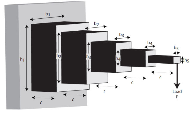
この例で示す問題は、段状の片持ち梁の設計に関するものです。特に、梁は規定の端部荷重に耐えることができなければなりません。最適化の問題は、さまざまなエンジニアリング設計の制約に従って梁の体積を最小化することです。

この問題はThanedarとVanderplaats [1]で説明されています。

段付き片持ち梁の設計問題

次の図に示すように、段付きの片持ち梁は一方の端で支えられ、自由端に荷重がかかります。梁は、サポートから一定の距離 $$L$$ で指定された荷重 $$P$$ を支えることができなければなりません。梁の設計者は、各ステップまたはセクションの幅 ($$b_i$$) と高さ ($$h_i$$) を変更できます。カンチレバーの各セクションの長さは同じで、$$l=L_1$$ です。

ビームの体積

梁の体積 $$V$$ は、個体のセクションの体積の合計です。

$$V=l(b_1{h}_1+b_2{h}_2+b_3{h}_3+b_4{h}_4+b_5{h}_5)$$.

設計上の制約:曲げ応力

座標の中心が梁の自由端の断面の中心にある、単一の片持ち梁を考えます。梁の点$$(x,y,z)$$における曲げ応力は次式で与えられる。

$${\sigma }_b=M(x)y/I$$,

ここで、$$M(x)$$ は $$x$$ における曲げモーメント、$$x$$ は端部荷重からの距離、$$I$$ は梁の面積モーメントです。

図に示す段付き片持ち梁では、梁の各セクションの最大モーメントは $$P{D}_i$$ です。ここで、$$D_i$$ は梁の各セクションの端部荷重 $$P$$ からの最大距離です。したがって、梁$${\sigma }_i$$のi番目のセクションの最大応力は次のように表される。

$${\sigma }_i=P{D}_i(h_i/2)/I_i$$,

最大応力は梁の端で発生します（$$y=h_i/2$$）。梁のi番目の断面の断面2次モーメントは次のように与えられる。

$$I_i=b_i{h}_i^3/12$$.

この式を$${\sigma }_i$$の式に代入すると、

$${\sigma }_i=6P{D}_i/b_i{h}_i^2$$.

カンチレバーの各部分の曲げ応力は、最大許容応力 $${\sigma }_{max}$$ を超えてはなりません。したがって、5 つの曲げ応力制約 (カンチレバーの各ステップに 1 つ) は次のようになります。

$$\frac{6Pl}{b_5{h}_5^2}\le {\sigma }_{max}$$

$$\frac{6P(2l)}{b_4{h}_4^2}\le {\sigma }_{max}$$

$$\frac{6P(3l)}{b_3{h}_3^2}\le {\sigma }_{max}$$

$$\frac{6P(4l)}{b_2{h}_2^2}\le {\sigma }_{max}$$

$$\frac{6P(5l)}{b_1{h}_1^2}\le {\sigma }_{max}$$

設計上の制約:端部たわみ

カスチリアーノの第二定理を使って片持ち梁の端のたわみを計算することができます。

$$\delta =\frac{\partial U}{\partial P}$$,

ここで、$$\delta$$ は梁のたわみ、$$U$$ は適用された力 $$P$$ により梁に蓄えられたエネルギーです。

片持ち梁に蓄えられたエネルギーは次のように表される。

$$U={\int }_0^L{M}^2/2EIdx$$,

ここで、$$M$$ は $$x$$ における適用された力のモーメントです。

片持ち梁の$$M=Px$$を考えると、前述の式は次のように書けます。

$$U=P^2/2E{\int }_0^l[(x+4l{)}^2/I_1+(x+3l{)}^2/I_2+(x+2l{)}^2/I_3+(x+l{)}^2/I_4+x^2/I_5]dx$$,

ここで、$$I_n$$ はカンチレバーの n 番目の部分の面積モーメントです。積分を評価すると$$U$$の式が得られる。

$$U=(P^2/2)(l^3/3E)(61/I_1+37/I_2+19/I_3+7/I_4+1/I_5)$$.

カスティリアーノの定理を適用すると、梁の端部のたわみは次のように表される。

$$\delta =P{l}^3/3E(61/I_1+37/I_2+19/I_3+7/I_4+1/I_5)$$.

片持ち梁の端部たわみ$$\delta$$は、最大許容たわみ$${\delta }_{max}$$より小さくなければなりません。これにより、制約が与えられます。

$$P{l}^3/3E(61/I_1+37/I_2+19/I_3+7/I_4+1/I_5)\le {\delta }_{max}$$.

設計上の制約:アスペクト比

カンチレバーの各ステップのアスペクト比は、最大許容アスペクト比 $$a_{max}$$ を超えてはなりません。つまり、

$$h_i/b_i\le a_{max}$$ ($$i=1,...,5$$)

設計上の制約:境界と整数制約

ビームの最初のステップは、最も近いセンチメートル単位でのみ機械加工できます。つまり、$$b_1$$ と $$h_1$$ は整数である必要があります。残りの変数は連続的です。変数の境界は次のとおりです。

$$1\le b_1\le 5$$

$$30\le h_1\le 65$$

$$2.4\le b_2,b_3\le 3.1$$

$$45\le h_2,h_3\le 60$$

$$1\le b_4,b_5\le 5$$

$$30\le h_4,h_5\le 65$$

この問題の設計パラメーター

この例の問題では、梁がサポートする必要がある端部荷重は $$P=50000N$$ です。

梁の長さと最大端部たわみは次のとおりです。

• ビーム全長、$$L=500cm$$

• 梁の個体のセクションの長さ、$$l=L_1=100cm$$

• 最大梁端たわみ、$${\delta }_{max}=2.7cm$$

梁の各ステップで許容される最大応力は $${\sigma }_{max}=14000N/c{m}^2$$ です。

梁の各段のヤング率は $$E=2\times 10^{7}N/c{m}^2$$ です。

問題ベースの設定

この問題の最適化変数を作成します。梁の最初のセクションの幅と高さの変数は整数型なので、連続する他の 4 つの変数とは別に作成する必要があります。

b1 = optimvar("b1","Type","integer","LowerBound",1,"UpperBound",5);
h1 = optimvar("h1","Type","integer","LowerBound",30,"UpperBound",65);
bc = optimvar("bc",4,"LowerBound",[2.4 2.4 1 1],"UpperBound",[3.1 3.1 5 5]);
hc = optimvar("hc",4,"LowerBound",[45 45 30 30],"UpperBound",[60 60 65 65]);

便宜上、高さと幅の変数を単一の変数に入れます。これらの変数を使用して、目的と制約を簡単に表現できます。

h = [h1;hc];
b = [b1;bc];

梁の体積を目的関数として最適化問題を作成します。梁の各ステップ (またはセクション) の長さは $$L_1=100$$ cm です: 体積 = $$L_1\sum h_i{w}_i$$。

L_1 = 100; % Length of each step of the cantilever
prob = optimproblem("Objective",L_1*dot(h,b));

応力に対する制約を作成します。

P = 50000; % End load
E = 2e7; % Young's modulus in N/cm^2
deltaMax = 2.7; % Maximum end deflection
sigmaMax = 14000; % Maximum stress in each section of the beam
aMax = 20; % Maximum aspect ratio in each section of the beam

stress = 6*P*L_1./(b.*(h.^2));
stepnum = (5:-1:1)';
stress = stress.*stepnum;
prob.Constraints.stress = stress <= sigmaMax;

たわみに対する制約を作成します。

deflectionMultiplier = (P*L_1^3/E)*[244 148 76 28 4];
bh3 = 1./(b.*(h.^3));
prob.Constraints.deflection = deflectionMultiplier*bh3 <= deltaMax;

アスペクト比の制約を作成します。

prob.Constraints.aspect = h <= aMax*b;

問題の設定を確認します。

show(prob)

  OptimizationProblem : 

	Solve for:
       b1, bc, h1, hc
	where:
       b1, h1 integer
	minimize :
       100*h1*b1 + 100*hc(1)*bc(1) + 100*hc(2)*bc(2) + 100*hc(3)*bc(3) + 100*hc(4)*bc(4)


	subject to stress:
       arg_LHS <= arg_RHS

       where:

             arg2 = zeros(5, 1);
             arg1 = zeros(5, 1);
             arg1(1) = h1;
             arg1(2:5) = hc;
             arg2(1) = b1;
             arg2(2:5) = bc;
             arg_LHS = ((30000000 ./ (arg2(:) .* arg1(:).^2)) .* extraParams{1});
             arg2 = 14000;
             arg1 = arg2(ones(1,5));
             arg_RHS = arg1(:);

       extraParams

	subject to deflection:
       arg_LHS <= 2.7

       where:

             arg2 = zeros(5, 1);
             arg1 = zeros(5, 1);
             arg1(1) = h1;
             arg1(2:5) = hc;
             arg2(1) = b1;
             arg2(2:5) = bc;
             arg_LHS = (extraParams{1} * (1 ./ (arg2(:) .* arg1(:).^3)));

       extraParams

	subject to aspect:
       -20*b1 + h1 <= 0
       -20*bc(1) + hc(1) <= 0
       -20*bc(2) + hc(2) <= 0
       -20*bc(3) + hc(3) <= 0
       -20*bc(4) + hc(4) <= 0

	variable bounds:
       1 <= b1 <= 5

       2.4 <= bc(1) <= 3.1
       2.4 <= bc(2) <= 3.1
         1 <= bc(3) <=   5
         1 <= bc(4) <=   5

       30 <= h1 <= 65

       45 <= hc(1) <= 60
       45 <= hc(2) <= 60
       30 <= hc(3) <= 65
       30 <= hc(4) <= 65

問題を解く

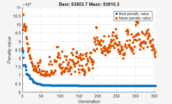
オプションを設定して、中程度の母集団サイズ 150、中程度の最大世代数 400、デフォルトのエリート数よりわずかに大きい 10、小さな関数許容値 1e-8、反復中の関数値を表示するプロット関数を使用します。

opts = optimoptions(@ga, ...
                    'PopulationSize', 150, ...
                    'MaxGenerations', 400, ...
                    'EliteCount', 10, ...
                    'FunctionTolerance', 1e-8, ...
                    'PlotFcn', @gaplotbestf);

ga ソルバーとオプションを指定して問題を解きます。

rng default % For reproducibility
[sol,fval,exitflag] = solve(prob,"Solver","ga","Options",opts)

Solving problem using ga.

ga stopped because the average change in the penalty function value is less than options.FunctionTolerance and 
the constraint violation is less than options.ConstraintTolerance.

sol = struct with fields:
    b1: 3
    bc: [4×1 double]
    h1: 60
    hc: [4×1 double]

fval = 
6.3804e+04

exitflag = 
    SolverConvergedSuccessfully

ソリューション変数とその境界を表示します。

widths = [sol.b1;sol.bc];
heights = [sol.h1;sol.hc];
widthbounds = [b1.LowerBound b1.UpperBound;
    bc.LowerBound bc.UpperBound];
heightbounds = [h1.LowerBound h1.UpperBound;
    hc.LowerBound hc.UpperBound];
T = table(widths,heights,widthbounds,heightbounds,...
    'VariableNames',["Width" "Height" "Width Bounds" "Height Bounds"])

T=5×4 table
    Width     Height    Width Bounds    Height Bounds
    ______    ______    ____________    _____________

         3        60       1      5       30    65   
    2.9063    54.983     2.4    3.1       45    60   
    2.5805    51.609     2.4    3.1       45    60   
    2.2785    45.565       1      5       30    65   
    1.7502    34.991       1      5       30    65   

解はどの境界にも存在しません。最初のソリューション変数は、指定されたとおり整数値になります。

離散非整数変数制約を追加する

エンジニアが、カンチレバーの 2 段目と 3 段目では、幅と高さを標準セットからのみ選択できることを知ったとします。この制約を追加すると、問題は[1]で解決された問題と同一になります。

まず、最適化に追加する追加の制約を定義します。

• 梁の2段目と3段目の幅は、[2.4、2.6、2.8、3.1]cmから選択する必要があります。

• 梁の2段目と3段目の高さは、[45、50、55、60]cmから選択する必要があります。

この問題を解決するには、変数 $$wc(1)$$、$$wc(2)$$、$$hc(1)$$、および $$hc(2)$$ を離散変数として指定する必要があります。理想的には、離散値として $$S(x_j)$$ を使用します。ここで、$$S$$ は許容される値のセットを表し、$$x_j$$ は問題の変数を表します。ただし、最適化変数をインデックスとして使用することはできません。この問題は、fcn2optimexpr を呼び出すことによって回避できます。

widthlist = [2.4,2.6,2.8,3.1];
heightlist = [45 50 55 60];
b23 = optimvar("w23",2,"Type","integer",...
    "LowerBound",1,"UpperBound",length(widthlist));
h23 = optimvar("h23",2,"Type","integer",...
    "LowerBound",1,"UpperBound",length(heightlist));
b45 = optimvar("b45",2,"LowerBound",1,"UpperBound",5);
h45 = optimvar("h45",2,"LowerBound",30,"UpperBound",65);
% Preferred syntax is we = [widthlist(b23(1));widthlist(b23(2))];
% However, this syntax is illegal.
% Instead call fcn2optimexpr.
we = fcn2optimexpr(@(x)[widthlist(x(1));widthlist(x(2))],b23);
he = fcn2optimexpr(@(x)[heightlist(x(1));heightlist(x(2))],h23);

先ほどと同じように、変数を表す式 b と h を作成します。

b = [b1;we;b45];
h = [h1;he;h45];

問題の残りの定式化は前と同じです。

prob2 = optimproblem("Objective",L_1*dot(h,b));

応力に対する制約を作成します。

stress = 6*P*L_1./(b.*(h.^2));
stepnum = (5:-1:1)';
stress = stress.*stepnum;
prob2.Constraints.stress = stress <= sigmaMax;

たわみに対する制約を作成します。

deflectionMultiplier = (P*L_1^3/E)*[244 148 76 28 4];
bh3 = 1./(b.*(h.^3));
prob2.Constraints.deflection = deflectionMultiplier*bh3 <= deltaMax;

アスペクト比の制約を作成します。

prob2.Constraints.aspect = h <= aMax*b;

問題の設定を確認します。

show(prob2)

  OptimizationProblem : 

	Solve for:
       b1, b45, h1, h23, h45, w23
	where:
       b1, h1, h23, w23 integer
	minimize :
       (100 .* (arg2(:).' * arg4(:)))

       where:

           arg4 = zeros(5, 1);
           arg2 = zeros(5, 1);
           anonymousFunction2 = @(x)[heightlist(x(1));heightlist(x(2))];
           arg1 = anonymousFunction2(h23);
           arg2(1) = h1;
           arg2(2:3) = arg1;
           arg2(4:5) = h45;
           anonymousFunction1 = @(x)[widthlist(x(1));widthlist(x(2))];
           arg3 = anonymousFunction1(w23);
           arg4(1) = b1;
           arg4(2:3) = arg3;
           arg4(4:5) = b45;


	subject to stress:
       arg_LHS <= arg_RHS

       where:

             arg4 = zeros(5, 1);
             arg2 = zeros(5, 1);
             anonymousFunction2 = @(x)[heightlist(x(1));heightlist(x(2))];
             arg1 = anonymousFunction2(h23);
             arg2(1) = h1;
             arg2(2:3) = arg1;
             arg2(4:5) = h45;
             anonymousFunction1 = @(x)[widthlist(x(1));widthlist(x(2))];
             arg3 = anonymousFunction1(w23);
             arg4(1) = b1;
             arg4(2:3) = arg3;
             arg4(4:5) = b45;
             arg_LHS = ((30000000 ./ (arg4(:) .* arg2(:).^2)) .* extraParams{1});
             arg2 = 14000;
             arg1 = arg2(ones(1,5));
             arg_RHS = arg1(:);

       extraParams

	subject to deflection:
       arg_LHS <= 2.7

       where:

             arg4 = zeros(5, 1);
             arg2 = zeros(5, 1);
             anonymousFunction2 = @(x)[heightlist(x(1));heightlist(x(2))];
             arg1 = anonymousFunction2(h23);
             arg2(1) = h1;
             arg2(2:3) = arg1;
             arg2(4:5) = h45;
             anonymousFunction1 = @(x)[widthlist(x(1));widthlist(x(2))];
             arg3 = anonymousFunction1(w23);
             arg4(1) = b1;
             arg4(2:3) = arg3;
             arg4(4:5) = b45;
             arg_LHS = (extraParams{1} * (1 ./ (arg4(:) .* arg2(:).^3)));

       extraParams

	subject to aspect:
       arg_LHS <= arg_RHS

       where:

             arg1 = zeros(5, 1);
             arg1(1) = h1;
             anonymousFunction2 = @(x)[heightlist(x(1));heightlist(x(2))];
             arg2 = anonymousFunction2(h23);
             arg1(2:3) = arg2;
             arg1(4:5) = h45;
             arg_LHS = arg1(:);
             arg2 = zeros(5, 1);
             anonymousFunction1 = @(x)[widthlist(x(1));widthlist(x(2))];
             arg1 = anonymousFunction1(w23);
             arg2(1) = b1;
             arg2(2:3) = arg1;
             arg2(4:5) = b45;
             arg_RHS = (20 .* arg2(:));

	variable bounds:
       1 <= b1 <= 5

       1 <= b45(1) <= 5
       1 <= b45(2) <= 5

       30 <= h1 <= 65

       1 <= h23(1) <= 4
       1 <= h23(2) <= 4

       30 <= h45(1) <= 65
       30 <= h45(2) <= 65

       1 <= w23(1) <= 4
       1 <= w23(2) <= 4

離散変数制約の問題を解く

ga ソルバーとオプションを指定して問題を解きます。

rng default % For reproducibility
[sol2,fval2,exitflag2] = solve(prob2,"Solver","ga","Options",opts)

Solving problem using ga.

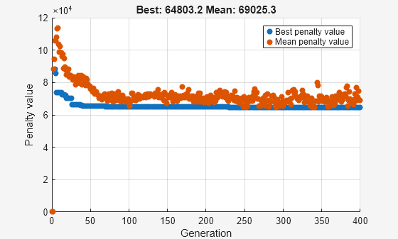
ga stopped because it exceeded options.MaxGenerations.

sol2 = struct with fields:
     b1: 3
    b45: [2×1 double]
     h1: 60
    h23: [2×1 double]
    h45: [2×1 double]
    w23: [2×1 double]

fval2 = 
6.4803e+04

exitflag2 = 
    SolverLimitExceeded

制約を追加すると目的が増加するだけなので、目的の値が増加します。

解を表示し、その境界と比較します。

widths = [sol2.b1;widthlist(sol2.w23(1));widthlist(sol2.w23(2));sol2.b45];
heights = [sol2.h1;heightlist(sol2.h23(1));heightlist(sol2.h23(2));sol2.h45];
widthbounds = [b1.LowerBound b1.UpperBound;
    widthlist(1) widthlist(end);
     widthlist(1) widthlist(end);
    b45.LowerBound b45.UpperBound];
heightbounds = [h1.LowerBound h1.UpperBound;
     heightlist(1) heightlist(end);
     heightlist(1) heightlist(end);
    h45.LowerBound h45.UpperBound];
T = table(widths,heights,widthbounds,heightbounds,...
    'VariableNames',["Width" "Height" "Width Bounds" "Height Bounds"])

T=5×4 table
    Width     Height    Width Bounds    Height Bounds
    ______    ______    ____________    _____________

         3        60       1      5       30    65   
       3.1        55     2.4    3.1       45    60   
       2.6        50     2.4    3.1       45    60   
     2.286     45.72       1      5       30    65   
    1.8532    34.004       1      5       30    65   

制限を受ける唯一のソリューション変数は 2 番目のセクションの幅で、これは最大値の 3.1 です。

参考文献

[1] Thanedar、P.B.、および G.N. Vanderplaats。"Survey of Discrete Variable Optimization for Structural Design." Journal of Structural Engineering 121 (3), 1995, pp. 301–306.

参考

ga | fcn2optimexpr | solve

トピック

• 遺伝的アルゴリズムを用いた混合整数エンジニアリング設計問題の解決