Single Period Goal-Based Wealth Management
This example shows a method for goal-based wealth management (GBWM). In GBWM, risk is not necessarily measured using the standard deviation, the value-at-risk, or any other common risk measure. Instead, risk is understood as the likelihood of not attaining an investor's goal. You choose a weight allocation that is on the traditional mean-variance efficient frontier and that also maximizes the probability of exceeding a wealth goal at the end of the investment horizon. In other words, you choose the portfolio on the efficient frontier that minimizes the risk of not attaining the investor's goal.
A common issue after computing the mean-variance efficient frontier is how to choose a single portfolio to invest in. This portfolio could be the maximum Sharpe ratio portfolio, which selects the weights that achieve the highest return given the amount of risk taken. However, choosing this portfolio does not take the investor's preferences into account. Another way strategy is to gauge the risk preference of the investor and select a portfolio that achieves a risk no larger than the investor's preferred risk. However, it is difficult to quantify the risk aversion of an investor. In this example, you use the probability of achieving a wealth goal to help choose a portfolio on the efficient frontier.
Load Data
Load the data and then annualize the asset returns and the variance-covariance matrix.
% Load data
load BlueChipStockMoments.mat
AssetMean = 12*AssetMean;
AssetCovar = 12*AssetCovar;
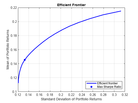
Plot Efficient Frontier
Use Portfolio to create a Portfolio object and estimateMaxSharpeRatio to compute the maximum Sharpe ratio. Then, use plotFrontier to plot the efficient frontier for long-only, fully-invested portfolios and mark the maximum Sharpe ratio portfolio.
% Create a Portfolio object.
p = Portfolio(AssetList=AssetList,AssetMean=AssetMean,...
    AssetCovar=AssetCovar);

% Add long-only, fully-invested constraints
p = setDefaultConstraints(p);

% Compute the maximum Sharpe ratio portfolio.
wSR = estimateMaxSharpeRatio(p);

% Plot the efficient frontier.
numPorts = 20;
figure;
[pret,prisk] = plotFrontier(p,20);
hold on
plot(estimatePortRisk(p,wSR),estimatePortReturn(p,wSR),'b.',...
    'MarkerSize',20);
legend('Efficient frontier','Max Sharpe Ratio',...
    'Location','southeast')
hold off
Choose Single Portfolio Using GBWM
GBWM provides a way to choose a single portfolio on the efficient frontier that allows you to incorporate the investor's preference in a straightforward way. In this case, the investor's goal is to reach a target wealth from their initial wealth at the end of the investment period . Therefore, you can formulate the problem as choosing the portfolio that maximizes the probability of having a wealth at time that surpasses the goal , while making sure that the chosen weights are on the efficient frontier.
% Define investor's preferences
W0 = 100;
G = 200;
T = 10;
For this example, assume that the wealth evolves following a Brownian motion [1]
,
where is a standard normal random variable.
The approach in this example also assumes that the returns follow a stationary distribution. In other words, the approach assumes that the returns have the same expectation and covariance throughout the investment period. The term “single-period” refers to the fact that the optimal allocation is computed only once at the beginning of the investment horizon assuming that the allocations will remain constant. This is a “set-it-and-forget-it” strategy. Although you can recompute the allocation weights at each reinvestment period by updating the time horizon and initial wealth, a single-period problem does not consider possible allocation changes in the middle of the investment horizon. In contrast, the optimal solution for a "multi-period" approach takes into account possible changes to the weights at intermediate investment periods. Thus, instead of just selecting the initial portfolio weights, multi-period problems compute the optimal strategy that should be followed given the changes in wealth at each of the reinvestment periods. The Dynamic Portfolio Allocation in Goal-Based Wealth Management for Multiple Time Periods example shows a multi-period version of the problem in this example.
Define Objective Function and Solve Problem
Find the portfolio that maximizes the probability of achieving the investor's goal given the prior assumptions. Maximizing is equivalent to minimizing , so the objective function is rewritten as
.
Since the relationship of and to the weights is represented by equality constraints in the problem, you can substitute these values in the objective function and remove the equality constraints that show the relationship between these three variables.
Define the objective function handle using the definition above and then use estimateCustomObjectivePortfolio to solve the problem.
% Define objective function
probability = @(w) normcdf(1/sqrt(T*(w'*p.AssetCovar*w)) * ...
    (log(G/W0) - (p.AssetMean'*w - (w'*p.AssetCovar*w)/2)*T));

% Solve problem
wGBWM = estimateCustomObjectivePortfolio(p,probability);
Plot Efficient Frontier
Use plotFrontier to plot the efficient frontier, the maximum Sharpe ratio portfolio, and the portfolio that maximizes the probability of achieving the goal (called the GBWM portfolio).
% Plot the efficient frontier.
figure;
plotFrontier(p,pret,prisk);
hold on
plot(estimatePortRisk(p,wSR),estimatePortReturn(p,wSR),'b.', ...
    'MarkerSize',20);
plot(estimatePortRisk(p,wGBWM),estimatePortReturn(p,wGBWM),'r.', ...
    'MarkerSize',20);
legend('Efficient frontier','Maximum Sharpe ratio', ...
    'GBWM Portfolio','Location','southeast')
hold off

The GBWM portfolio is riskier than the maximum Sharpe ratio portfolio. This extra risk is necessary to maximize the probability of attaining the investor's wealth goal by time .
Compare GBWM Portfolio to Maximum Sharpe Ratio Portfolio
Compare the probabilities of achieving the wealth goal by the end of the investment period for the maximum Sharpe ratio portfolio against the GBWM portfolio.
Tprobabilities = table(1-probability(wSR),1-probability(wGBWM),...
    RowNames={'P(W_T >= G)'},VariableNames={'SR','GBWM'})
Tprobabilities=1×2 table
                     SR        GBWM
                   _______    _______

    P(W_T >= G)    0.94592    0.95347
The probability of successfully meeting the investor's wealth goal does not change much between the maximum Sharpe ratio portfolio and the GBWM portfolio. Using this information, an investor can understand the trade-off between achieving their wealth goal by time compared to choosing a less risky portfolio. For example, an investor might choose a minimum variance portfolio that has a much lower probability of achieving their wealth goal by time . Find the minimum variance (MV) portfolio, and compare the probability of achieving the wealth goal using this portfolio with the other two approaches.
wMV = estimateFrontierLimits(p,'min');
Tprobabilities.MV = 1-probability(wMV)Tprobabilities=1×3 table
SR GBWM MV
_______ _______ ______
P(W_T >= G) 0.94592 0.95347 0.8252
References
[1] Das, Sanriv R., Daniel Ostrov, Anand Radhakrishnan, and Deep Srivastav. “A New Approach to Goals-Based Wealth Management.” Journal of Investment Management. 16, no. 3 (2018): 1–27.
See Also
Portfolio | estimatePortSharpeRatio | estimateFrontier | estimateFrontierByReturn | estimateFrontierByRisk | estimateCustomObjectivePortfolio
Topics
- Dynamic Portfolio Allocation in Goal-Based Wealth Management for Multiple Time Periods
- Multiperiod Goal-Based Wealth Management Using Reinforcement Learning
- Diversify Portfolios Using Custom Objective
- Portfolio Optimization Against a Benchmark
- Solver Guidelines for Custom Objective Problems Using Portfolio Objects