designFracDelayFIR

Design and implement band-limited fractional delay FIR filter

Since R2021a

Syntax

h = designFracDelayFIR

h = designFracDelayFIR(Name=Value)

[h,i0] = designFracDelayFIR(___)

[h,i0,MBW] = designFracDelayFIR(___)

Description

h = designFracDelayFIR designs a fractional delay FIR filter of length 50 and delay 0.5. The output h is the vector of filter coefficients.

h = designFracDelayFIR(Name=Value) specifies options using one or more name-value arguments. (since R2024a)

For example, h = designFracDelayFIR(FractionalDelay=0.3,Bandwidth=0.6) designs a fractional delay FIR filter of delay 0.3. The function automatically determines the appropriate FIR length N for which the combined bandwidth is at least 0.6. As the SystemObject argument is true, the function returns a dsp.FIRFilter object.

When you specify any of the numeric input arguments in single precision, the function designs the filter coefficients in single precision. Alternatively, you can use the Datatype and like arguments to control the coefficients data type. (since R2024b)

[h,i0] = designFracDelayFIR(___) also returns the integer latency i0 of the FIR filter. This value is approximately equal to N/2, where N is the length of the filter. The nominal group delay of the filter is i0+fd, where fd is the fractional delay of the filter.

[h,i0,MBW] = designFracDelayFIR(___) also returns the measured combined bandwidth of the filter h.

Examples

Design Fractional Delay FIR Filter by Using Delay and Filter Length

Design a fractional delay FIR filter using the designFracDelayFIR function. Pass the delay and the filter length as the input arguments to the function. Vary the filter length and observe the effect on the measured combined bandwidth and the nominal group delay.

Vary Filter Length

Set delay to 0.25 and filter length to 8 and design the fractional delay FIR filter.

fd = 0.25;
[h1,i10,bw1] = designFracDelayFIR(FractionalDelay=fd,FilterLength=8)

h1 = 1×8

   -0.0086    0.0417   -0.1355    0.8793    0.2931   -0.0968    0.0341   -0.0074

i10 = 
3

bw1 = 
0.5810

The nominal group delay of the filter i10+fd equals 3.25 samples. The measured combined bandwidth of the filter is 0.5810 in normalized frequency units.

Repeat the process with a filter length of 32 taps.

[h2,i20,bw2] = designFracDelayFIR(FractionalDelay=fd,FilterLength=32)

h2 = 1×32

   -0.0001    0.0004   -0.0009    0.0017   -0.0029    0.0046   -0.0071    0.0104   -0.0148    0.0208   -0.0291    0.0410   -0.0594    0.0926   -0.1752    0.8983    0.2994   -0.1252    0.0758   -0.0515    0.0367   -0.0266    0.0193   -0.0139    0.0098   -0.0067    0.0044   -0.0028    0.0016   -0.0009    0.0004   -0.0001

i20 = 
15

bw2 = 
0.8571

The nominal group delay of the filter now equals 15.25 samples. By increasing the filter length, the integer latency i0 increases, resulting in an increase in the nominal group delay. The combined bandwidth of the filter also increases to 0.8571 in normalized frequency units.

Increase the filter length to 64 taps. The group delay increases to 31.25 samples, and the integer latency is 31 samples. The measured combined bandwidth of the filter further increases to 0.9219, covering 92.19% of the overall bandwidth. As the filter length continues to increase, the combined bandwidth tends closer towards 1.

[h3,i30,bw3] = designFracDelayFIR(FractionalDelay=fd,FilterLength=64)

h3 = 1×64

   -0.0000    0.0001   -0.0001    0.0002   -0.0003    0.0004   -0.0006    0.0008   -0.0010    0.0013   -0.0017    0.0022   -0.0027    0.0034   -0.0042    0.0051   -0.0061    0.0074   -0.0088    0.0105   -0.0125    0.0149   -0.0177    0.0212   -0.0255    0.0311   -0.0386    0.0494   -0.0664    0.0979   -0.1787    0.8997    0.2999   -0.1277    0.0801   -0.0575    0.0442   -0.0352    0.0288   -0.0239    0.0200   -0.0168    0.0142   -0.0120    0.0101   -0.0085    0.0071   -0.0059    0.0049   -0.0040

i30 = 
31

bw3 = 
0.9219

Plot Magnitude Response

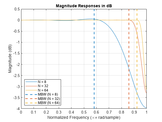
Plot the magnitude response of the three filters. Mark the measured combined bandwidth (MBW) of the three filters. By increasing the filter length, you can see that the measured combined bandwidth increases.

[H1,w] = freqz(h1,1);
H2 = freqz(h2,1);
H3 = freqz(h3,1);
figure;
plot(w/pi,mag2db(abs([H1 H2 H3])))
hold on
hline = lines;
xline(bw1, LineStyle = '--', LineWidth = 2, Color = hline(1,:))
xline(bw2, LineStyle = '--', LineWidth = 2, Color = hline(2,:))
xline(bw3, LineStyle = '--', LineWidth = 2, Color = hline(3,:))
hold off
title('Magnitude Responses in dB')
xlabel("Normalized Frequency (\times\pi rad/sample)")
ylabel("Magnitude (dB)")
grid
 
legend('N = 8','N = 32','N = 64',...
       'MBW (N = 8)',...
       'MBW (N = 32)',...
       'MBW (N = 64)',Location='southwest')

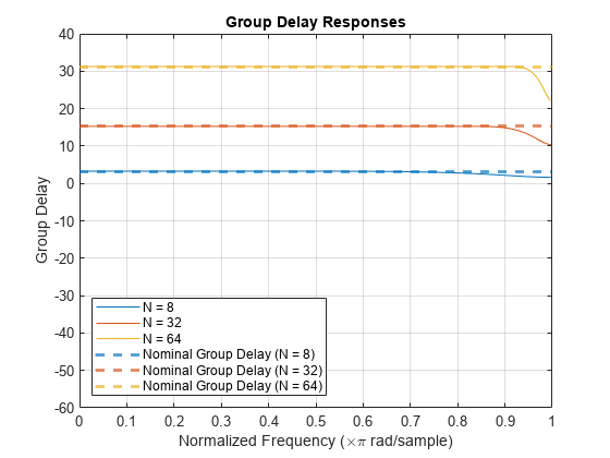
Plot Group Delay Response

Plot the group delay response of the three filters. Mark the nominal group delay i0 + fd of the three filters. By increasing the filter length, you can see that the nominal group delay increases.

[g1,w] = grpdelay(h1,1);
g2 = grpdelay(h2,1);
g3 = grpdelay(h3,1);

figure;
plot(w/pi,[g1 g2 g3])

 
hline = lines;
yline(i10+fd, LineStyle = '--', LineWidth = 2, Color = hline(1,:))
yline(i20+fd, LineStyle = '--', LineWidth = 2, Color = hline(2,:))
yline(i30+fd, LineStyle = '--', LineWidth = 2, Color = hline(3,:))

 
title('Group Delay Responses')

xlabel("Normalized Frequency (\times\pi rad/sample)")
ylabel("Group Delay")
grid
 
legend('N = 8','N = 32','N = 64',...
        'Nominal Group Delay (N = 8)',...
       'Nominal Group Delay (N = 32)',...
      'Nominal Group Delay (N = 64)',Location='southwest');
ylim([-60,40]);

Design Fractional Delay FIR Filter by Using Delay and Combined Bandwidth

Design a fractional delay FIR filter using the designFracDelayFIR function. Pass the delay and the combined bandwidth as input arguments to the function.

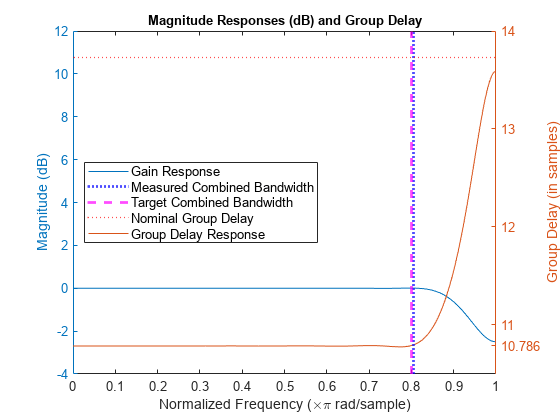
Set delay to 0.786 and the target combined bandwidth to be 0.8. The function designs a filter that has a length of 22 taps, an integer latency i0 of 10 samples, and a combined bandwidth mbw of 0.8044 in normalized frequency units. This mbw value results in a combined bandwidth coverage of 80.44% of the frequency domain and exceeds the specified target combined bandwidth. The nominal group delay of the filter i0+fd equals 10.786.

fd  = 0.786;
tbw = 0.8;
[h,i0,mbw] = designFracDelayFIR(FractionalDelay=fd,Bandwidth=tbw)

h = 1×22

    0.0003   -0.0011    0.0026   -0.0052    0.0094   -0.0156    0.0248   -0.0386    0.0611   -0.1052    0.2512    0.9225   -0.1548    0.0769   -0.0455    0.0281   -0.0173    0.0102   -0.0057    0.0028   -0.0012    0.0003

i0 = 
10

mbw = 
0.8044

Plot the impulse response of the FIR.

stem((0:length(h)-1),h); 
xlabel('h'); ylabel('h[n]');
title('Impulse Response of the Fractional Delay FIR')

Plot the resulting magnitude response and the group delay response. Mark the nominal group delay and the combined bandwidth of the filter.

[H1,w] = freqz(h,1);
G1 = grpdelay(h,1);
figure;
yyaxis left
plot(w/pi,mag2db(abs(H1)))
ylabel("Magnitude (dB)")

hold on
yyaxis right
plot(w/pi,G1)
ylabel("Group Delay (in samples)")

hline = lines;
xline(mbw, LineStyle =':',  Color = 'b', LineWidth = 2)
xline(tbw, LineStyle = '--', Color = 'm', LineWidth = 2)
yline(i0+fd, LineStyle = ':', Color = 'r', LineWidth = 1)
yticks([i0, i0+fd,i0+1:i0+9]); 

hold off
title('Magnitude Responses (dB) and Group Delay', FontSize = 10)
xlabel("Normalized Frequency (\times\pi rad/sample)")

legend('Gain Response','Group Delay Response','Measured Combined Bandwidth',...
        'Target Combined Bandwidth','Nominal Group Delay', ...
        Location = 'west', FontSize = 10)

Design Fractional Delay FIR Filter and Compare with Shifted Input

Design a fractional delay FIR filter using the designFracDelayFIR function. Determine the group delay of the designed filter. Create a dsp.FIRFilter object that uses these designed coefficients and hence has the same group delay. Alternately, create a sampled sequence of a known function. Pass the sampled sequence to the FIR filter. Compare the output of the FIR filter to the shifted samples of the known function. Specify this shift to be equal to the group delay of the FIR filter. Verify that the two sequences match.

Set the delay of the FIR filter to 1/3 and the length to 6 taps.

fd = 1/3;
len = 6;

Design the filter using the designFracDelayFIR function and determine the center index i0 and the combined bandwidth bw of the filter. The group delay of this filter is i0 + fd or approximately 2.33 for the bandwidth of bw. To design the filter in single-precision, use the Datatype or like argument. Alternatively, you can specify any of the numerical arguments in single-precision.

[h,i0,bw] = designFracDelayFIR(FractionalDelay=fd,...
    FilterLength=len,Datatype="single")

h = 1x6 single row vector

    0.0293   -0.1360    0.7932    0.3966   -0.1088    0.0257

i0 = single

2

bw = single

0.5158

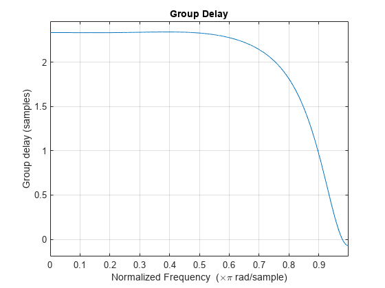
Create a dsp.FIRFilter object and set its numerator to the filter coefficients h. This filter is now effectively a fractional delay FIR filter. Verify that the group delay response of this filter is approximately 2.33 for the duration of the bandwidth bw.

fdf = dsp.FIRFilter(h);
grpdelay(fdf)

Compare with Shifted Function

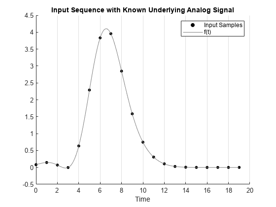
Define a sequence x as samples of a known function.

f = @(t) (0.1*t.^2+cos(0.9*t)).*exp(-0.1*(t-5).^2);
n = (0:19)'; t = linspace(0,19,512);
x = f(n); % Samples

Plot the sampled values x against the original known function f(t).

scatter(n,x,20,'k','filled');
hold on;
plot(t,f(t),'color',[0.5 0.5 0.5],'LineWidth',0.5)
hold off;
xlabel('Time')
legend(["Input Samples","f(t)"])
title('Input Sequence with Known Underlying Analog Signal')
ax = gca; ax.XGrid='on';

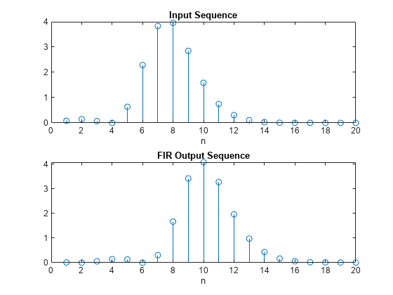
Pass the sampled sequence x through the FIR filter. Plot the input sequence and output sequence.

y = fdf(x);

subplot(2,1,1);
stem(x);
title('Input Sequence');
xlabel('n')
subplot(2,1,2)
stem(y);
title('FIR Output Sequence');
xlabel('n')

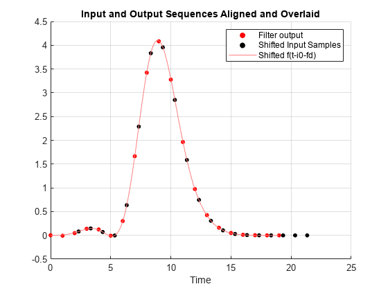
Shift the input sequence horizontally by i0 + fd, which is equal to the group delay of the FIR filter. Plot the function f(t-i0-FD). Verify that the input and output sequences fall roughly on the shifted function.

figure
scatter(n,y,20,'red','filled')
hold on;
scatter(n+i0+fd,x,20,'black','filled')
plot(t,f(t-i0-fd),'Color',[1,0.5,0.5],'LineWidth',0.1)
xlabel('Time')
legend(["Filter output","Shifted Input Samples","Shifted f(t-i0-fd)"])
hold off
grid on
title('Input and Output Sequences Aligned and Overlaid')

Input Arguments

Name-Value Arguments

Specify optional pairs of arguments as Name1=Value1,...,NameN=ValueN, where Name is the argument name and Value is the corresponding value. Name-value arguments must appear after other arguments, but the order of the pairs does not matter.

Example: designFracDelayFIR(FractionalDelay=0.4,Bandwidth=0.8,SystemObject=true) designs and returns a dsp.FIRFilter object.

FractionalDelay — Fractional delay of filter

0.5 | positive scalar in the range [0,1]

Fractional delay of the filter, specified as a positive scalar in the range [0,1]. The fractional delay value that you specify determines the measured combined bandwidth MBW of the filter.

When you set FractionalDelay to 0 or 1, the designed filter has a full bandwidth.

Data Types: single | double

FilterLength — Length of FIR filter

50 | integer greater than 1

Length of the fractional delay FIR filter, specified as an integer greater than 1.

Data Types: single | double | int8 | int16 | int32 | int64 | uint8 | uint16 | uint32 | uint64

Bandwidth — Target combined bandwidth

positive scalar less than 0.999

Target combined bandwidth, specified as a positive scalar less than 0.999. This is the value of the combined bandwidth that the function must satisfy. Combined bandwidth is defined as the minimum of the gain bandwidth and the group delay bandwidth.

Specifying both filter length and target combined bandwidth results in an overdetermined design. The function does not support specifying both the values. When you specify the target combined bandwidth, the function determines the corresponding filter length, and designs the filter accordingly.

Specify a higher target combined bandwidth for a longer filter. For example, setting Bandwidth to 0.9 yields a filter of length of 52, while increasing Bandwidth to 0.99 yields a length of 724, which is more than 10 times longer. As Bandwidth tends towards 1, the filter length theoretically tends towards infinity.

Data Types: single | double

Datatype — Data type of filter coefficients by type name

"double" (default) | "single"

Since R2024b

Data type of the filter coefficients, specified by type name as "double" or "single".

You can use the Dataype or the like argument to specify the data type of the filter coefficients, but you cannot use both arguments at the same time.

If you specify the data type of the filter coefficients using this argument, the function ignores the data types of the other numeric arguments.

Data Types: char | string

like — Data type of filter coefficients by prototype

real floating-point value

Since R2024b

Data type of the filter coefficients, specified as a prototype of a real floating-point value.

You can use the Dataype or the like argument to specify the data type of filter coefficients, but you cannot use both arguments at the same time.

If you specify the data type of the filter coefficients using this argument, the function ignores the data types of the other numeric arguments.

Example: B = designFracDelayFIR(FractionalDelay=fd,FilterLength=filtLen,like=single(filtLen))

Example: filtLen = single(64); B = designFracDelayFIR(FractionalDelay=fd,FilterLength=filtLen,like=filtLen)

Data Types: single | double

SystemObject — Option to create filter System object™

false (default) | true

Since R2024a

Option to create a filter System object, specified as one of these:

• false –– The function returns a vector of fractional delay FIR filter coefficients.

• true –– The function returns a dsp.FIRFilter System object.

Data Types: logical

Verbose — Option to print function call in MATLAB^®

false (default) | true

Option to print the entire function call in MATLAB, specified as one of these:

• false –– The function does not print the function call.

• true –– The function prints the entire function call including the default values of the Name=Value arguments that you did not specify when calling the function.

  Use this argument to view all the values used by the function to design and implement the filter.

Data Types: logical

Output Arguments

h — Designed filter

row vector | dsp.FIRFilter object

Designed filter, returned as one of these options.

• Fractional delay FIR filter coefficients –– The function returns a row vector of length N when you set the SystemObject argument to false.

  You can specify N through the FilterLength argument. If you specify the Bandwidth argument, the function treats this value as the desired combined bandwidth, determines the corresponding filter length, and designs the filter accordingly.

  When you use filter length to design the filter, and you specify single-precision values in any of the input arguments, the function outputs single-precision filter coefficients. (since R2024a)

  If you specify the data type using the Datatype or the like argument, the function ignores the data types of the other numeric arguments. (since R2024b)

• Multirate FIR filter object –– The function returns a dsp.FIRFilter object when you set the SystemObject argument to true.

Data Types: single | double

i0 — Integer latency

integer

Integer latency of the designed FIR filter, returned as an integer value. Integer latency is the smallest integer shift required to make the symmetric Kaiser window causal. This value is approximately equal to half the filter length or N/2. For more details, see Integer latency, i0.

The nominal group delay of the filter is given by i0+fd, where fd is the value you specify through the FractionalDelay argument.

If you specify the data type using the Datatype or the like argument, the function ignores the data types of the other numeric arguments. (since R2024b)

Data Types: single | double

MBW — Measured combined bandwidth

positive scalar less than 0.999

Measured combined bandwidth, returned as a real positive scalar less than 0.999. This is the value of the combined bandwidth of the designed filter. Combined bandwidth is defined as the minimum of gain bandwidth and group delay bandwidth.

The function designs the filter such that the measured combined bandwidth MBW meets or exceeds the target combined bandwidth. The function determines the filter length so that it meets the bandwidth constraint.

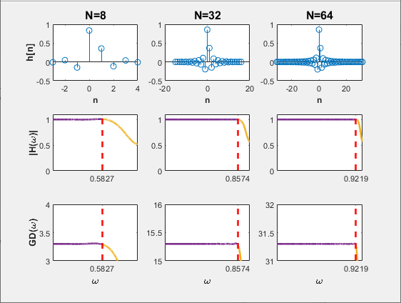
When you specify the filter length N, the function treats this value as the desired length of the filter. The measured combined bandwidth in this case varies with the length. Larger the value of N, higher is the measured combined bandwidth MBW. This plot shows the variation. As the filter length increases, the combined bandwidth of the filter moves closer towards 1. The red dashed vertical line marks the combined bandwidth for each length. The fractional delay value for each of these filters is 0.3

If you specify the data type using the Datatype or the like argument, the function ignores the data types of the other numeric arguments. (since R2024b)

Data Types: single | double

More About

Fractional Delay FIR Filter

The fractional delay FIR filter is an FIR approximation of an ideal sinc shift filter with a fractional (noninteger) delay value fd in the range [0,1].

The ideal shift filter models a band-limited D/A interpolator followed by shifted A/D uniform sampling. Assuming a uniform sampling rate and shift invariant interpolation, the resulting overall system can be expressed as a convolution filter, approximated by an FIR filter. In other words, $$y[n]=h_{fd}[n]\ast x[n]$$, which encapsulates the D/A interpolation, shift, and A/D sampling chain as depicted in the figure.

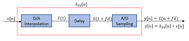
where,

$$\begin{array}{l}{h}_{fd}[n]=\mathrm{sinc}(n-fd),\\ \widehat{x}(t)={\displaystyle \sum _{k}x[k]\mathrm{sinc}(t-k)}\\ \Rightarrow \widehat{x}(t+fd)={\displaystyle \sum _{k}x[k]\mathrm{sinc}}\left(t+fd-k\right)\end{array}$$

The frequency response of the ideal shift filter is

$$H_{fd}(\omega )=e^{-j\omega fd}.$$

The ideal shift filter has a flat unity gain response, and a constant group delay of fd, where fd is the fractional delay value you specify through the FractionalDelay argument.

The function computes the FIR approximation by truncating the ideal filter and weighting the truncated filter by a Kaiser window.

$$\widehat{x}(n+fd)\approx y[n]=\left(h\ast x\right)\left[n\right],whereh[m]=\mathrm{sinc}(m+fd)·K_{N,\beta }[m]$$

where, $$K_{N,\beta }[m]$$ is a Kaiser window of length N and has a shape parameter β. The function designs the Kaiser window to optimize the FIR frequency response, maximizing the combined bandwidths of both gain response and group delay response.

To make the FIR approximation causal, the algorithm introduces an additional shift of i0, making the nominal group delay of the filter equal to i0+fd. The frequency response of the truncated filter is $$H(\omega )=e^{-j\omega \left(fd+i_0\right)}$$.

For more details, see Integer latency, i0.

Integer latency, i0

Integer latency, i0, is the smallest integer shift that is required to make the symmetric Kaiser window causal.

The ideal sinc shift filter is an allpass filter, which has an infinite and noncausal impulse response. To approximate this filter, the function uses a finite index Kaiser window of length N that is symmetric around the origin and captures the main lobe of the sinc function.

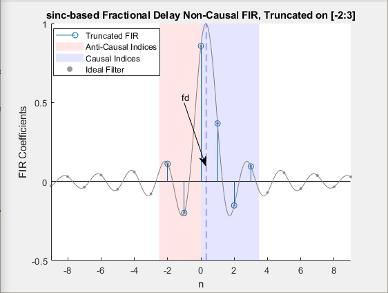
Due to the symmetric nature of the window, half of the window (approximately equal to N/2) is on the negative side of the origin making the truncated filter anti-causal. To make the truncated filter causal, shift the anti-causal (negative indices) part of the FIR window by an integer latency, i0, that is approximately equal to N/2.

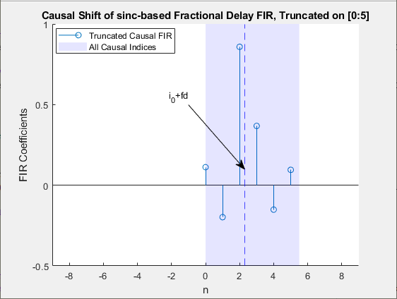
The overall delay of the causal FIR filter is i0+fd, where fd is the fractional delay.

For more details on FIR approximation, see the Causal FIR Approximations of an Ideal sinc Shift Filter section in Design Fractional Delay FIR Filters.

Gain Bandwidth

Given an FIR frequency response H(ω), the gain bandwidth is the largest interval [0 Ba] over which the gain response |H(ω)| is close to 1 up to a given tolerance value, tol.

$$B_a=\underset{\omega }{\max }\left\{\left|\left|H(\nu )\right|-1\right|<tol\forall 0\le \nu \le \omega \right\}$$

Group Delay Bandwidth

Given tolerance tol and group delay response G, the group delay bandwidth is the largest interval [0 Bg] such that the group delay is close to the nominal value fd.

$$B_g=\underset{\omega }{\max }\left\{\left|G(\nu )-fd-i_0\right|<tol\forall 0\le \nu \le \omega \right\}$$

Combined Bandwidth

Combined bandwidth is defined as the minimum between gain bandwidth and group delay bandwidth.

$$B_c=\min (B_a,B_g)$$

Combined bandwidth depends on the fractional delay fd and the length of the FIR filter N.

Extended Capabilities

C/C++ Code Generation

Generate C and C++ code using MATLAB® Coder™.

When you set the SystemObject argument to false, the function supports code generation with no limitations.

When you set the SystemObject argument to true, the inputs to the function must be constants when generating code. (since R2024a)

This function supports strict single precision in generated code. When you use filter length to design the filter, and you specify any of the input arguments in single-precision, or use the Datatype and like arguments to specify single-precision (since R2024b), the code you generate uses strictly single-precision arithmetic. (since R2024a)

Version History

Introduced in R2021a

R2024b: Specify data type of filter coefficients explicitly

You can now specify the data type of filter coefficients explicitly using the Datatype and like arguments.

R2024a: Value only syntax is discouraged

Starting in R2024a, specifying the arguments using the Value only syntax is discouraged in the designFractionalDelayFIR function.

Existing instances of the function using the Value only arguments continue to run but are discouraged. Instead, specify the arguments using the Name=Value syntax.

R2024a: Support for Name=Value syntax

Starting in R2024a, the designFractionalDelayFIR function supports specifying the input arguments using the Name=Value syntax.

Here is the table that shows how to replace your existing code.

Existing code	Replace with
designFractionalDelayFIR(fd)	designFractionalDelayFIR(FractionalDelay=fd)
designFractionalDelayFIR(fd,N) N is an integer greater than 1.	designFractionalDelayFIR(FractionalDelay=fd,FilterLength=N)
designFractionalDelayFIR(fd,TBW) TBW is a positive scalar less than 0.999.	designFractionalDelayFIR(FractionalDelay=fd,Bandwidth=TBW)

R2024a: Support for strict single precision

When you use filter length to design the filter, and you specify any of the input arguments in single-precision, the function designs filter coefficients in single precision both in simulation and in generated code.

R2024a: New 'SystemObject' argument

You can now generate a dsp.FIRFilter object from the designFracDelayFIR function by specifying the 'SystemObject' argument to true.

R2024a: Support for code generation when 'SystemObject' flag is true

The designFractionalDelayFIR function supports code generation when you set the 'SystemObject' flag to true.