音声合成の敵対的生成ネットワーク (GAN) の学習
この例では、敵対的生成ネットワーク (GAN) に学習させ、そのネットワークを使用して音声を生成する方法を説明します。
はじめに
敵対的生成ネットワークでは、ジェネレーターとディスクリミネーターが互いに競い合うことで、生成品質を向上させます。
GAN は、オーディオ処理および音声処理の分野で高い関心を集めました。応用例としては、テキスト音声合成、音声変換、音声強調などがあります。
この例では、GAN の教師なし学習を実行してオーディオ波形を合成します。この例の GAN はパーカッション音を生成します。話し声など、他の種類の音も、同じ方法で生成できます。
事前学習済みの GAN を使用したオーディオ合成
GAN にゼロから学習させる前に、事前学習済みの GAN ジェネレーターを使用してパーカッション音を合成します。
事前学習済みのジェネレーターをダウンロードします。
loc = matlab.internal.examples.downloadSupportFile("audio","examples/PercussiveSoundGenerator.zip");
unzip(loc,pwd)
サポート関数 synthesizePercussiveSound が、事前学習済みのネットワークを呼び出して、16 kHz でサンプリングされたパーカッション音を合成します。関数 synthesizePercussiveSound は、この例の最後に示されています。
パーカッション音を合成して再生します。
synthsound = synthesizePercussiveSound();

fs = 16e3;
sound(synthsound,fs)
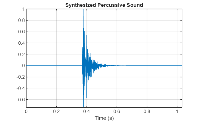
合成されたパーカッション音をプロットします。
t = (0:length(synthsound)-1)/fs;
plot(t,synthsound)
grid on
xlabel("Time (s)")
title("Synthesized Percussive Sound")
axis tight
パーカッション音シンセサイザーを使用して他のオーディオ エフェクトを適用することで、より複雑なアプリケーションを作成できます。たとえば、合成されたパーカッション音に残響を適用できます。
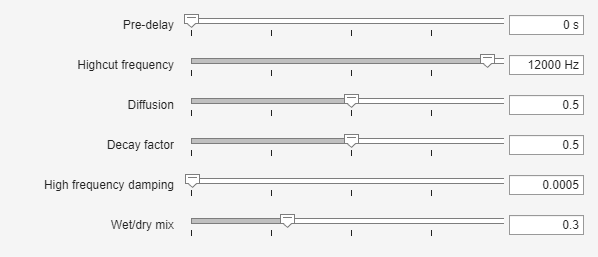
reverberator (Audio Toolbox)オブジェクトを作成し、そのパラメーター チューナー UI を開きます。シミュレーション実行時、この UI を使用して reverberator パラメーターを調整できます。
reverb = reverberator(SampleRate=fs,HighCutFrequency=12e3);
parameterTuner(reverb);
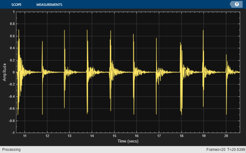
パーカッション音を可視化するtimescope (DSP System Toolbox)オブジェクトを作成します。
ts = timescope(SampleRate=fs, ...
    TimeSpanSource="Property", ...
    TimeSpanOverrunAction="Scroll", ...
    TimeSpan=10, ...
    BufferLength=10*256*64, ...
    ShowGrid=true, ...
    YLimits=[-1 1]);
ループ内で、パーカッション音を合成して残響を適用します。パラメーター チューナー UI を使用して残響を調整します。より長い時間シミュレーションを実行する場合は、loopCount パラメーターの値を大きくします。
loopCount = 20;
for ii = 1:loopCount
    synthsound = synthesizePercussiveSound;
    synthsound = reverb(gather(synthsound));
    ts(synthsound(:,1));
    soundsc(synthsound,fs)
    pause(0.5)
end
学習
事前学習済みのパーカッション音ジェネレーターの動作を確認できたので、次に、学習プロセスを詳しく見ていきます。
GAN は深層学習ネットワークの一種で、学習データと類似した特性をもつデータを生成します。
GAN は同時に学習させることが可能な 2 つのネットワーク、すなわち、"ジェネレーター" と "ディスクリミネーター" で構成されています。
ジェネレーター。ベクトルまたはランダムな値を入力として与えられ、このネットワークは学習データと同じ構造のデータを生成します。ディスクリミネーターを騙すのがジェネレーターの仕事です。
ディスクリミネーター。学習データと生成されたデータの両方の観測値を含むデータのバッチを与えられ、このネットワークはその観測値が実データか生成データかの分類を試みます。
ジェネレーターのパフォーマンスを最大化するには、生成されたデータが与えられたときのディスクリミネーターの損失を最大化します。つまり、ジェネレーターの目的はディスクリミネーターが実データと分類するようなデータを生成することです。ディスクリミネーターのパフォーマンスを最大化するには、実データと生成データ両方のバッチが与えられたときのディスクリミネーターの損失を最小化します。これらの方法によって、いかにも本物らしいデータを生成するジェネレーターと、学習データの特性である強い特徴表現を学習したディスクリミネーターを得ることが理想的な結果です。
この例では、パーカッション音を表す偽の時間-周波数短時間フーリエ変換 (STFT) を作成するようにジェネレーターに学習させます。STFT がジェネレーターによって合成されたものなのか、本物のオーディオ信号から計算されたものなのかを識別するように、ディスクリミネーターに学習させます。短時間録音した実際のパーカッション音の STFT を計算し、本物の STFT を作成します。

データのダウンロード
Freesound One-Shot Percussive Sounds データセット [2] で GAN に学習させます。データセットをダウンロードし、解凍します。ライセンスによって商用利用が禁止されているファイルを削除します。
url1 = "https://zenodo.org/record/4687854/files/one_shot_percussive_sounds.zip";
url2 = "https://zenodo.org/record/4687854/files/licenses.txt";
downloadFolder = tempdir;

percussivesoundsFolder = fullfile(downloadFolder,"one_shot_percussive_sounds");
licensefilename = fullfile(percussivesoundsFolder,"licenses.txt");
if ~datasetExists(percussivesoundsFolder)
    disp("Downloading Freesound One-Shot Percussive Sounds Dataset (112.6 MB) ...")
    unzip(url1,downloadFolder)
    websave(licensefilename,url2);
    removeRestrictiveLicense(percussivesoundsFolder,licensefilename)
end
データセットを指すaudioDatastore (Audio Toolbox)オブジェクトを作成します。
ads = audioDatastore(percussivesoundsFolder,IncludeSubfolders=true,OutputDataType="single");前処理パイプラインの定義
データストアにあるパーカッション音信号から、短時間フーリエ変換 (STFT) データを生成します。
STFT パラメーターを定義します。
fftLength = 256;
win = hann(fftLength,"periodic");
overlapLength = 128;
hopLength = numel(win) - overlapLength;
STFT のホップ数が片側変換のビンの数と等しくなるように、必要なオーディオ信号長を導出します。後ほど、片側変換に偶数個のビンが含まれるように強制します。
numHops = fftLength/2;
signalLength = numel(win) + (numHops-1)*hopLength;
データストアに変換を追加し、目的のサンプル レートになるようにオーディオを再サンプリングし、目的の長さになるようにオーディオのサイズを変更し、オーディオを必ずモノラルにするには、サポート関数 preprocessAudio を使用します。
tads = transform(ads,@(x,xinfo)preprocessAudio(x,xinfo,signalLength),IncludeInfo=true);
片側 STFT の振幅を計算するための変換をデータストアに追加します。
tads = transform(tads,@(x){abs(stft(x,Window=win,OverlapLength=overlapLength,FrequencyRange="onesided"))});readall を呼び出して、データをメモリに抽出します。可能な場合は並列プールを使用して処理を高速化します。
STrain = readall(tads,UseParallel=canUseParallelPool);
Starting parallel pool (parpool) using the 'Processes' profile ...
21-Oct-2024 11:21:05: Job Queued. Waiting for parallel pool job with ID 1 to start ...
Connected to parallel pool with 6 workers.
出力は、各要素が STFT である cell 配列として返されます。STFT を 4 番目の次元に沿って連結します。
STrain = cat(4,STrain{:});人間の知覚に合わせるため、データを対数スケールに変換します。
STrain = log(STrain + 1e-6);
片側スペクトルが偶数になるように強制します。
isOddLengthHalfsided = rem(size(STrain,1),2)~=0;
if isOddLengthHalfsided
    STrain = STrain(1:end-1,:,:,:);
end
学習セットのサイズを検査します。
numBands = size(STrain,1)
numBands =
128
numHops = size(STrain,2)
numHops =
128
numSignals = size(STrain,4)
numSignals =
9839
平均値が 0、標準偏差が 1 となるように学習データを正規化します。
STFT 内の各周波数ビンの平均と標準偏差を計算します。
SMean = mean(STrain,[2 3 4]);
SStd = std(STrain,1,[2 3 4]);
各周波数ビンを正規化します。
STrain = (STrain - SMean)./SStd;
[1] の方法に従い、スペクトルを 3 の標準偏差にクリッピングしてから [-1 1] に再スケーリングし、データを有界にします。
STrain = STrain/3;
STrain = clip(STrain,-1,1);
学習データを反復処理するための arrayDatastore を作成します。
ads = arrayDatastore(STrain,IterationDimension=4);
学習ループでバッチを処理するための minibatchqueue を作成します。
miniBatchSize = 256;
mbq = minibatchqueue(ads,MiniBatchSize=miniBatchSize,MiniBatchFormat="SSBC");
ジェネレーター モデルの定義
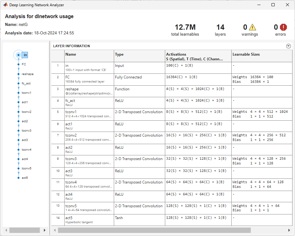
パーカッション音の STFT を生成するネットワークを定義します。このネットワークは、100 個の要素から成る潜在ベクトルを受け取り、全結合層、およびそれに続く形状変更層と、活性化層をもつ一連の転置畳み込み層を使用して、それらを 128 行 128 列の配列にアップサンプリングします。
ジェネレーターの入力の長さを指定します。
numLatentInputs = 100;
モデルのパラメーターを指定します。ジェネレーターのアーキテクチャは [1] の表 4 で定義されています。
initialSize = [4,4];
filterSize = [4,4];
numFilters = [512,256,128,64,1];
numConvLayers = numel(numFilters);
numStride = [2,2];
FC1sizeControl = 1024;
FC1size = prod(initialSize)*FC1sizeControl;
ジェネレーターが実際の信号から抽出されたのと同じサイズのスペクトログラムを出力することを確認します。
expFinalSize = [numBands,numHops]
expFinalSize = 1×2

    128    128
actFinalSize = initialSize.*numStride.^numConvLayers
actFinalSize = 1×2

    128    128
ネットワークを層のシーケンスとして構築します。
layers = [
    inputLayer([numLatentInputs,1],"CB",Name="in")

    fullyConnectedLayer(FC1size,Name="FC")
    functionLayer(@(x)dlarray(reshape(stripdims(x),initialSize(1),initialSize(2),FC1sizeControl,size(x,2)),"SSCB"), ...
        Formattable=true,Acceleratable=true,Name="reshape")
    reluLayer(Name="fc_act")

    transposedConv2dLayer(filterSize,numFilters(1),Stride=numStride,Cropping="same",Name="tconv1")
    reluLayer(Name="act1")

    transposedConv2dLayer(filterSize,numFilters(2),Stride=numStride,Cropping="same",Name="tconv2")
    reluLayer(Name="act2")

    transposedConv2dLayer(filterSize,numFilters(3),Stride=numStride,Cropping="same",Name="tconv3")
    reluLayer(Name="act3")

    transposedConv2dLayer(filterSize,numFilters(4),Stride=numStride,Cropping="same",Name="tconv4")
    reluLayer(Name="act4")

    transposedConv2dLayer(filterSize,numFilters(5),Stride=numStride,Cropping="same",Name="tconv5")
    tanhLayer(Name="act5")];

netG = dlnetwork(layers);
ジェネレーター ネットワークを解析します。
analyzeNetwork(netG)
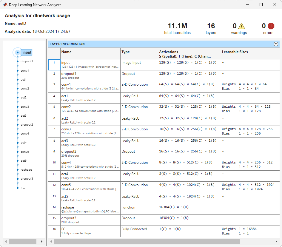
ディスクリミネーター モデルの定義
STFT を実際のものまたは生成されたものとして分類するネットワークを構築します。このネットワークは、128×128 のイメージを受け取り、leaky ReLU 層をもつ一連の畳み込み層とそれに続く全結合層を使用してスカラーの予測スコアを出力します。このディスクリミネーターのアーキテクチャは [1] の表 5 で定義されています。ディスクリミネーターがジェネレーターを圧倒しないように、ドロップアウトを含めます。
dropoutProb = 0.2;
scale = 0.2;
numFiltersD = [numFilters(end-1:-1:1),FC1sizeControl];

layersDiscriminator = [
    imageInputLayer([numBands,numHops],Name="input")

    dropoutLayer(dropoutProb,Name="dropout1")

    convolution2dLayer(filterSize,numFiltersD(1),Stride=numStride,Padding="same",Name="conv1")
    leakyReluLayer(scale,Name="act1")

    convolution2dLayer(filterSize,numFiltersD(2),Stride=numStride,Padding="same",Name="conv2")
    leakyReluLayer(scale,Name="act2")

    convolution2dLayer(filterSize,numFiltersD(3),Stride=numStride,Padding="same",Name="conv3")
    leakyReluLayer(scale,Name="act3")

    dropoutLayer(dropoutProb,Name="dropout2")

    convolution2dLayer(filterSize,numFiltersD(4),Stride=numStride,Padding="same",Name="conv4")
    leakyReluLayer(scale,Name="act4")

    convolution2dLayer(filterSize,numFiltersD(5),Stride=numStride,Padding="same",Name="conv5")
    leakyReluLayer(scale,Name="act5")

    functionLayer(@(x)dlarray(reshape(stripdims(x),FC1size,size(x,4)),"CB"), ...
        Acceleratable=true,Formattable=true,Name="reshape")

    dropoutLayer(dropoutProb,Name="dropout3")

    fullyConnectedLayer(1,Name="FC")
    ];
netD = dlnetwork(layersDiscriminator );
ディスクリミネーター ネットワークを解析します。
analyzeNetwork(netD)
学習オプションの定義
学習するエポック数を指定します。
maxEpochs = 500;
データを使い切るのに必要な反復回数を計算します。
numIterationsPerEpoch = floor(size(STrain,4)/miniBatchSize);
Adam 最適化のオプションを指定します。ジェネレーターとディスクリミネーターの学習率を 0.0002 に設定します。どちらのネットワークも、勾配の減衰係数に 0.5 を、2 乗勾配の減衰係数に 0.999 を使用します。
learnRateGenerator = 0.0002;
learnRateDiscriminator = 0.0002;
gradientDecayFactor = 0.5;
squaredGradientDecayFactor = 0.999;
モデルの学習
Adam のパラメーターを初期化します。
trailingAvgGenerator = [];
trailingAvgSqGenerator = [];
trailingAvgDiscriminator = [];
trailingAvgSqDiscriminator = [];
saveCheckpoints を true に設定すると、10 エポックごとに dlnetwork を MAT ファイルに保存できます。学習が中断された場合、この MAT ファイルを使用して学習を再開できます。
saveCheckpoints =  true;
true;学習を高速化するには、dlaccelerate を使用します。
discriminatorGradients_acc = dlaccelerate(@discriminatorGradients);
generatorGradients_acc = dlaccelerate(@generatorGradients);
学習の進行状況を監視するには、trainingProgressMonitor を使用します。
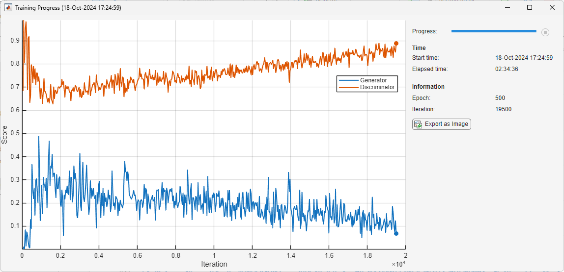
monitor = trainingProgressMonitor( ...
   Metrics=["Generator","Discriminator"], ...
   Info=["Epoch","Iteration"], ...
   XLabel="Iteration");

groupSubPlot(monitor,Score=["Generator","Discriminator"])
カスタム学習ループを使用して GAN に学習させます。実行には数時間かかることがあります。
各エポックで、学習データをシャッフルしてデータのミニバッチについてループします。
iteration = 0;

for epoch = 1:maxEpochs

    % Shuffle the data
    shuffle(mbq);

    % Loop over mini-batches.
    while hasdata(mbq) && ~monitor.Stop
        iteration = iteration + 1;

        % Read mini-batch of data.
        X = next(mbq);
        thisBatchSize = size(X,finddim(X,'B'));


        % DISCRIMINATOR
        % Generate latent inputs for the generator network.
        Z = createGeneratorSeed(numLatentInputs,thisBatchSize);

        % Calculate discriminator loss and gradients
        [lossD,gradientsD,scoreD] = dlfeval(discriminatorGradients_acc,netG,netD,X,Z);

        % Update the discriminator network parameters.
        [netD,trailingAvgDiscriminator,trailingAvgSqDiscriminator] = adamupdate(netD,gradientsD, ...
            trailingAvgDiscriminator,trailingAvgSqDiscriminator,iteration, ...
            learnRateDiscriminator,gradientDecayFactor,squaredGradientDecayFactor);


        % GENERATOR
        % Generate latent inputs for the generator network.
        Z = createGeneratorSeed(numLatentInputs,thisBatchSize);

        % Calculate generator loss and gradients
        [lossG,gradientsG,scoreG] = dlfeval(generatorGradients_acc,netG,netD,Z);

        % Update the generator network parameters.
        [netG,trailingAvgGenerator,trailingAvgSqGenerator] = adamupdate(netG,gradientsG, ...
            trailingAvgGenerator,trailingAvgSqGenerator,iteration, ...
            learnRateGenerator,gradientDecayFactor,squaredGradientDecayFactor);

    end

    % Every 10 epochs, save a training snapshot to a MAT file.
    if mod(epoch,10)==0
        if saveCheckpoints
            % Save checkpoint in case training is interrupted.
            save("audiogancheckpoint.mat", ...
                "netG","netD","iteration");
        end
    end

    % Update the training progress monitor.
    recordMetrics(monitor,iteration, ...
        Generator=mean(scoreG.extractdata(),'all'), ...
        Discriminator=mean(scoreD.extractdata(),'all'));

    updateInfo(monitor,Epoch=epoch,Iteration=iteration);
    monitor.Progress = min(100*(iteration/(numIterationsPerEpoch*maxEpochs)),100);
end
モデルの評価
ネットワークの学習が完了したので、次に、合成プロセスをさらに詳しく見ていきます。

学習済みのパーカッション音ジェネレーターは、乱数値の入力配列から短時間フーリエ変換 (STFT) 行列を合成します。逆 STFT (ISTFT) 演算は、時間-周波数の STFT を時間領域の合成オーディオ信号に変換します。
このジェネレーターは、乱数値のベクトルを入力として受け取ります。サンプルの入力ベクトルを生成します。
Z = createGeneratorSeed(numLatentInputs,1);
ランダム ベクトルをジェネレーターに渡し、STFT イメージを作成します。
XGenerated = predict(netG,Z);
STFT の dlarray を単精度行列に変換し、絶対値の最大値が 1 になるように再スケーリングします。
Shalf = extractdata(XGenerated);
Shalf = Shalf./max(abs(Shalf),[],'all');
学習用の STFT を生成するのに使用した正規化とスケーリングの手順を逆にたどり、元の状態に戻します。
Shalf = 3*Shalf;
Shalf = (Shalf.*SStd) + SMean;
STFT を、対数領域から線形領域に変換します。
Shalf = exp(Shalf);
生成されたスペクトルに片側スペクトルの最後のビンが含まれていない場合は、それをゼロとして追加します。
if isOddLengthHalfsided
    Shalf = cat(1,Shalf,zeros(1,size(Shalf,2)));
end
STFT を、片側から両側に変換します。
if rem(fftLength,2)==0
    S = [Shalf;Shalf((end-1):-1:2,:)];
else
    S = [Shalf;Shalf(end:-1:2,:)];
end
STFT 行列には位相情報が含まれていません。stftmag2sig を使用して信号の位相を推定し、オーディオ サンプルを生成します。
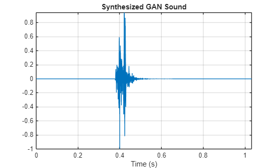
myAudio = stftmag2sig(S,fftLength, ...
    FrequencyRange="twosided", ...
    Window=win, ...
    OverlapLength=overlapLength, ...
    MaxIterations=20, ...
    Method="fgla");
myAudio = myAudio./max(abs(myAudio),[],"all");
合成されたパーカッション音を再生します。
fs = 16000;
sound(myAudio,fs)
合成されたパーカッション音をプロットします。
t = (0:length(myAudio)-1)/fs;
plot(t,myAudio)
grid on
xlabel("Time (s)")
title("Synthesized GAN Sound")
axis tight
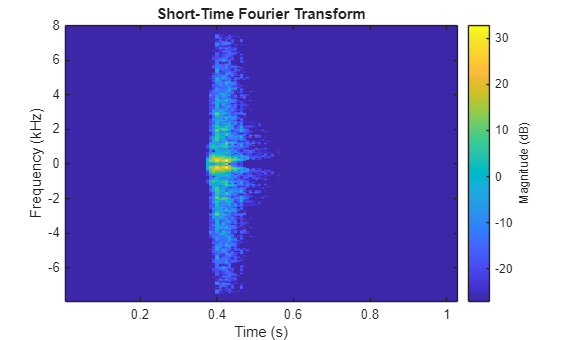
合成されたパーカッション音の STFT をプロットします。
figure
stft(myAudio,fs,Window=win,OverlapLength=overlapLength);
サポート関数
ジェネレーターのシードの作成
function Z = createGeneratorSeed(numLatentInputs,miniBatchSize)
Z = dlarray(2*(rand(numLatentInputs,miniBatchSize,"single") - 0.5 ),'CB');
if canUseGPU
    Z = gpuArray(Z);
end
end
ディスクリミネーターの勾配
function [lossD,gradientsD,scoreD] = discriminatorGradients(netG,netD,X,Z)
% Calculate the predictions for real data with the discriminator network.
X = X./max(abs(X),[],[1,2]); % ~Scale invariance
YReal  = forward(netD,X);

% Calculate the predictions for generated data with the discriminator network.
XGenerated = forward(netG,Z);
XGenerated = XGenerated./max(abs(XGenerated),[],[1,2]); % ~Scale invariance
YGenerated = forward(netD,XGenerated);

lossD = discriminatorLoss(YReal,YGenerated);

gradientsD = dlgradient(lossD,netD.Learnables);

scoreD = 0.5*(mean(sigmoid(YReal)) + mean((1 - sigmoid(YGenerated)))); % A measure of how much the discriminator was correct

end
ジェネレーターの勾配
function [lossG,gradientsG,scoreG] = generatorGradients(netG,netD,Z)

% Calculate the predictions for generated data with the discriminator network.
XGenerated = forward(netG,Z);
XGenerated = XGenerated./max(abs(XGenerated),[],[1,2]); % ~Scale invariance
YGenerated = forward(netD,XGenerated);

% Discriminator and Generator loss
lossG = generatorLoss(YGenerated);

% For each network, calculate the gradients with respect to the loss.
gradientsG = dlgradient(lossG,netG.Learnables);

scoreG = mean(sigmoid(YGenerated)); % A measure of how much the generator was fooled.
end
ディスクリミネーターの損失
function lossD = discriminatorLoss(YReal,YGenerated)
fake = dlarray(zeros(1,size(YReal,2)));
real = dlarray(ones(1,size(YReal,2)));

lossD = (mean(sigmoid_cross_entropy_with_logits(YGenerated,fake)) + ...
    mean(sigmoid_cross_entropy_with_logits(YReal,real))) / 2;
end
ジェネレーターの損失
function lossG = generatorLoss(YGenerated)
real = dlarray(ones(1,size(YGenerated,2)));
lossG = mean(sigmoid_cross_entropy_with_logits(YGenerated,real));
end
ロジットを使用したシグモイド クロス エントロピー
function out = sigmoid_cross_entropy_with_logits(x,z)
out = max(x,0) - x .* z + log(1 + exp(-abs(x)));
end
オーディオの前処理
function [out,xinfo] = preprocessAudio(in,xinfo,signalLength)
% Ensure mono
in = mean(in,2);

% Resample to 16 kHz
x = resample(in,16e3,xinfo.SampleRate);

% Force to the desired signal length
y = resize(x,signalLength,Side="both");

% Scale
out = y./max(abs(y));

end
制限付きライセンスの削除
function removeRestrictiveLicense(percussivesoundsFolder,licensefilename)

% Parse the licenses file that maps ids to license. Create a table to hold the info.
f = fileread(licensefilename);
K = jsondecode(f);
fns = fields(K);
T = table(Size=[numel(fns),4], ...
    VariableTypes=["string","string","string","string"], ...
    VariableNames=["ID","FileName","UserName","License"]);
for ii = 1:numel(fns)
    fn = string(K.(fns{ii}).name);
    li = string(K.(fns{ii}).license);
    id = extractAfter(string(fns{ii}),"x");
    un = string(K.(fns{ii}).username);
    T(ii,:) = {id,fn,un,li};
end

% Remove any files that prohibit commercial use. Find the file inside the
% appropriate folder, and then delete it.
unsupportedLicense = "http://creativecommons.org/licenses/by-nc/3.0/";
fileToRemove = T.ID(strcmp(T.License,unsupportedLicense));
for ii = 1:numel(fileToRemove)
    fileInfo = dir(fullfile(percussivesoundsFolder,"**",fileToRemove(ii)+".wav"));
    delete(fullfile(fileInfo.folder,fileInfo.name))
end

end
パーカッション音の合成
function y = synthesizePercussiveSound

persistent pGenerator pMean pSTD
if isempty(pGenerator)
    % If the MAT file does not exist, download it
    filename = "PercussiveSoundGenerator.mat";
    load(filename,"SMean","SStd","netG");
    pMean = SMean;
    pSTD  = SStd;
    pGenerator = netG;
end

Z = createGeneratorSeed(100,1);

% Pass the random vector to the generator to create an STFT image.
XGenerated = predict(pGenerator,Z);

% Convert the STFT dlarray to a single-precision matrix.
Shalf = extractdata(XGenerated);

% Rescale.
Shalf = Shalf./max(abs(Shalf),[],'all');

% Revert the normalization and scaling steps used to generate the
% STFTs for training.
Shalf = 3*Shalf;
Shalf = (Shalf.*pSTD) + pMean;

% Convert the STFT from the log domain to the linear domain.
Shalf = exp(Shalf);

% The generated spectrum doesn't include the final bin of a
% half-sided spectrum. Add it back as zeros.
Shalf = cat(1,Shalf,zeros(1,size(Shalf,2)));

% Convert the STFT from one-sided to two-sided.
S = [Shalf;Shalf((end-1):-1:2,:)];

% The STFT matrix does not contain any phase information. Use stftmag2sig
% to estimate the signal phase and produce audio samples.
myAudio = stftmag2sig(S,256, ...
    FrequencyRange="twosided", ...
    Window=hann(256,"periodic"), ...
    OverlapLength=128, ...
    MaxIterations=20, ...
    Method="fgla");

% Rescale to a max absolute value of 1.
y = myAudio./max(abs(myAudio),[],"all");
end
参考文献
[1] Donahue, C., J. McAuley, and M. Puckette. 2019."Adversarial Audio Synthesis." ICLR.
[2] Ramires, Antonio, Pritish Chandna, Xavier Favory, Emilia Gomez, and Xavier Serra. "Neural Percussive Synthesis Parameterised by High-Level Timbral Features." "ICASSP 2020 - 2020 IEEE International Conference on Acoustics, Speech and Signal Processing (ICASSP)", 2020. https://doi.org/10.1109/icassp40776.2020.9053128.