Speaker Diarization Using x-vectors
Speaker diarization is the process of partitioning an audio signal into segments according to speaker identity. It answers the question "who spoke when" without prior knowledge of the speakers and, depending on the application, without prior knowledge of the number of speakers.
Speaker diarization has many applications, including: enhancing speech transcription by structuring text according to active speaker, video captioning, content retrieval (what did Jane say?) and speaker counting (how many speakers were present in the meeting?).
In this example, you perform speaker diarization using a pretrained x-vector system [1] to characterize regions of audio and agglomerative hierarchical clustering (AHC) to group similar regions of audio [2]. To see how the x-vector system was defined and trained, see Speaker Recognition Using x-vectors (Audio Toolbox).
Download Pretrained Speaker Diarization System
Download the pretrained speaker diarization system and supporting files. The total size is approximately 22 MB.
downloadFolder = matlab.internal.examples.downloadSupportFile("audio","SpeakerDiarization.zip");
dataFolder = tempdir;
unzip(downloadFolder,dataFolder)
netFolder = fullfile(dataFolder,"SpeakerDiarization");

addpath(netFolder)
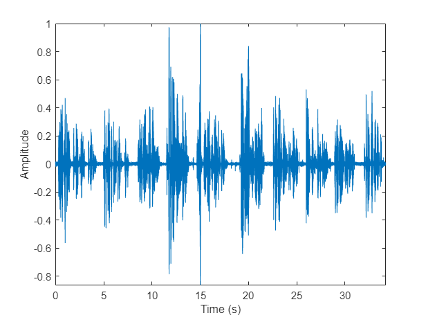
Load an audio signal and a table containing ground truth annotations. The signal consists of five speakers. Listen to the audio signal and plot its time-domain waveform.
[audioIn,fs] = audioread("exampleconversation.flac");
load("exampleconversationlabels.mat","groundTruth")
audioIn = audioIn./max(abs(audioIn));
sound(audioIn,fs)

t = (0:size(audioIn,1)-1)/fs;

figure(1)
plot(t,audioIn)
xlabel("Time (s)")
ylabel("Amplitude")
axis tight
Extract x-vectors
In this example, you used a pretrained x-vector system based on [1]. To see how the x-vector system was defined and trained, see Speaker Recognition Using x-vectors (Audio Toolbox).
Load Pretrained x-Vector System
Load the lightweight pretrained x-vector system. The x-vector system consists of:
afe- anaudioFeatureExtractor(Audio Toolbox) object to extract mel frequency cepstral coefficients (MFCCs).factors- a struct containing the mean and standard deviation of MFCCs determined from a representative data set. These factors are used to standardize the MFCCs.dlnet- a traineddlnetwork. The network is used to extract x-vectors from the MFCCs.projMat- a trained projection matrix to reduce the dimensionality of x-vectors.plda- a trained PLDA model for scoring x-vectors.
xvecsys = load("xvectorSystem.mat");Extract Standardized Acoustic Features
Extract standardized MFCC features from the audio data. View the feature distributions to confirm that the standardization factors learned from a separate data set approximately standardize the features derived in this example. A standard distribution has a mean of zero and a standard deviation of 1.
features = single((extract(xvecsys.afe,audioIn)-xvecsys.factors.Mean')./xvecsys.factors.STD');

figure(2)
histogram(features)
xlabel("Standardized MFCC")
Extract x-Vectors
Each acoustic feature vector represents approximately 0.01 seconds of audio data. Group the features into approximately 2 second segments with 0.1 second hops between segments.
featureVectorHopDur = (numel(xvecsys.afe.Window) - xvecsys.afe.OverlapLength)/xvecsys.afe.SampleRate; segmentDur =2; segmentHopDur =
0.1; segmentLength = round(segmentDur/featureVectorHopDur); segmentHop = round(segmentHopDur/featureVectorHopDur); idx = 1:segmentLength; featuresSegmented = []; while idx(end) < size(features,1) featuresSegmented = cat(3,featuresSegmented,features(idx,:)); idx = idx + segmentHop; end
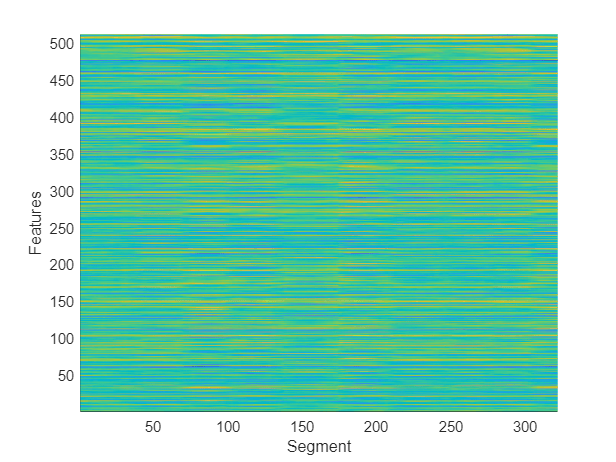
Extract x-vectors from each segment. x-vectors correspond to the output from the first fully-connected layer in the x-vector model trained in Speaker Recognition Using x-vectors (Audio Toolbox). The first fully-connected layer is the first segment-level layer after statistics are calculated for the time-dilated frame-level layers. Visualize the x-vectors over time.
xvecs = zeros(512,size(featuresSegmented,3));
for sample = 1:size(featuresSegmented,3)
    dlX = dlarray(featuresSegmented(:,:,sample),"TCB");
    xvecs(:,sample) = predict(xvecsys.dlnet,dlX,Outputs="fc_1");
end

figure(3)
surf(xvecs',EdgeColor="none")
view([90,-90])
axis([1 size(xvecs,1) 1 size(xvecs,2)])
xlabel("Features")
ylabel("Segment")
Apply the pretrained linear discriminant analysis (LDA) projection matrix to reduce the dimensionality of the x-vectors and then visualize the x-vectors over time.
x = xvecsys.projMat*xvecs;

figure(4)
surf(x',EdgeColor="none")
view([90,-90])
axis([1 size(x,1) 1 size(x,2)])
xlabel("Features")
ylabel("Segment")

Cluster x-vectors
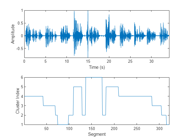
An x-vector system learns to extract compact representations (x-vectors) of speakers. Cluster the x-vectors to group similar regions of audio using either agglomerative hierarchical clustering (clusterdata (Statistics and Machine Learning Toolbox)) or k-means clustering (kmeans (Statistics and Machine Learning Toolbox)). [2] suggests using agglomerative hierarchical clustering with PLDA scoring as the distance measurement. K-means clustering using a cosine similarity score is also commonly used. Assume prior knowledge of the number of speakers in the audio. Set the maximum clusters to the number of known speakers + 1 so that the background is clustered independently.
knownNumberOfSpeakers = numel(unique(groundTruth.Label)); maxclusters = knownNumberOfSpeakers + 1; clusterMethod ='agglomerative - PLDA scoring'; switch clusterMethod case "agglomerative - PLDA scoring" T = clusterdata(x',Criterion="distance",distance=@(a,b)helperPLDAScorer(a,b,xvecsys.plda),linkage="average",maxclust=maxclusters); case "agglomerative - CSS scoring" T = clusterdata(x',Criterion="distance",distance="cosine",linkage="average",maxclust=maxclusters); case "kmeans - CSS scoring" T = kmeans(x',maxclusters,Distance="cosine"); end
Plot the cluster decisions over time.
figure(5)
tiledlayout(2,1)

nexttile
plot(t,audioIn)
axis tight
ylabel("Amplitude")
xlabel("Time (s)")

nexttile
plot(T)
axis tight
ylabel("Cluster Index")
xlabel("Segment")
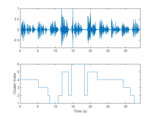
To isolate segments of speech corresponding to clusters, map the segments back to audio samples. Plot the results.
mask = zeros(size(audioIn,1),1);
start = round((segmentDur/2)*fs);

segmentHopSamples = round(segmentHopDur*fs);

mask(1:start) = T(1);
start = start + 1;
for ii = 1:numel(T)
    finish = start + segmentHopSamples;
    mask(start:start + segmentHopSamples) = T(ii);
    start = finish + 1;
end
mask(finish:end) = T(end);

figure(6)
tiledlayout(2,1)

nexttile
plot(t,audioIn)
axis tight

nexttile
plot(t,mask)
ylabel("Cluster Index")
axis tight
xlabel("Time (s)")
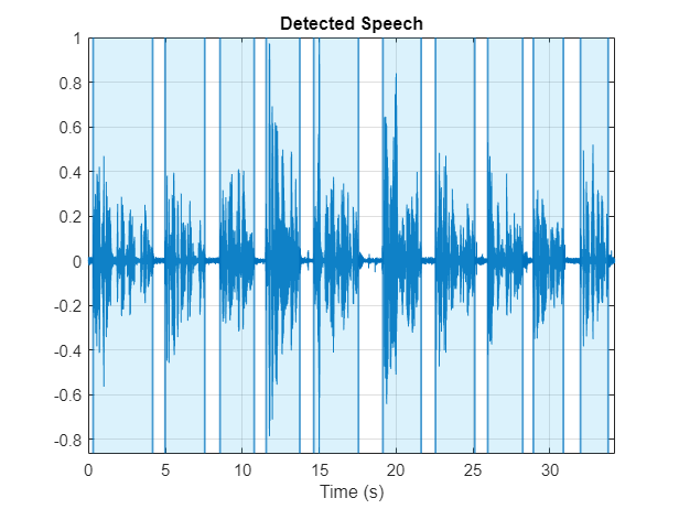
Use detectSpeech (Audio Toolbox) to determine speech regions. Use sigroi2binmask (Signal Processing Toolbox) to convert speech regions to a binary voice activity detection (VAD) mask. Call detectSpeech a second time without any arguments to plot the detected speech regions.
mergeDuration = 0.5;
VADidx = detectSpeech(audioIn,fs,MergeDistance=fs*mergeDuration);

VADmask = sigroi2binmask(VADidx,numel(audioIn));

figure(7)
detectSpeech(audioIn,fs,MergeDistance=fs*mergeDuration)
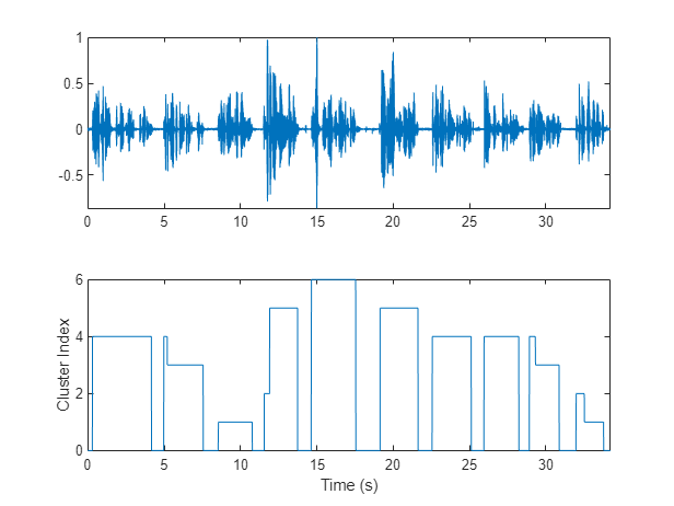
Apply the VAD mask to the speaker mask and plot the results. A cluster index of 0 indicates a region of no speech.
mask = mask.*VADmask;

figure(8)
tiledlayout(2,1)

nexttile
plot(t,audioIn)
axis tight

nexttile
plot(t,mask)
ylabel("Cluster Index")
axis tight
xlabel("Time (s)")
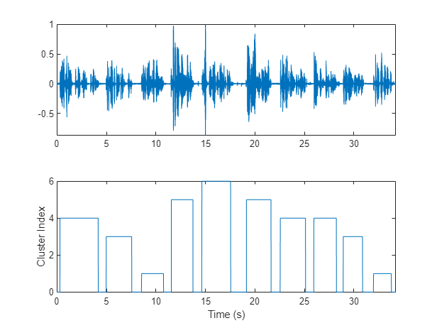
In this example, you assume each detected speech region belongs to a single speaker. If more than two labels are present in a speech region, merge them to the most frequently occurring label.
maskLabels = zeros(size(VADidx,1),1);
for ii = 1:size(VADidx,1)
    maskLabels(ii) = mode(mask(VADidx(ii,1):VADidx(ii,2)),"all");
    mask(VADidx(ii,1):VADidx(ii,2)) = maskLabels(ii);
end

figure(9)
tiledlayout(2,1)

nexttile
plot(t,audioIn)
axis tight

nexttile
plot(t,mask)
ylabel("Cluster Index")
axis tight
xlabel("Time (s)")
Count the number of remaining speaker clusters.
uniqueSpeakerClusters = unique(maskLabels);
numSpeakers = numel(uniqueSpeakerClusters)
numSpeakers =
5
Visualize Diarization Results
Create a signalMask (Signal Processing Toolbox) object and then plot the speaker clusters. Label the plot with the ground truth labels. The cluster labels are color coded with a key on the right of the plot. The true labels are printed above the plot.
msk = signalMask(table(VADidx,categorical(maskLabels)));

figure(10)
plotsigroi(msk,audioIn,true)
axis([0 numel(audioIn) -1 1])

trueLabel = groundTruth.Label;
for ii = 1:numel(trueLabel)
    text(VADidx(ii,1),1.1,trueLabel(ii),FontWeight="bold")
end

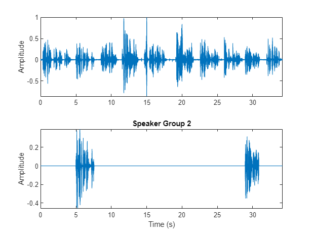
Choose a cluster to inspect and then use binmask (Signal Processing Toolbox) to isolate the speaker. Plot the isolated speech signal and listen to the speaker cluster.
speakerToInspect =2; cutOutSilenceFromAudio =
true; bmsk = binmask(msk,numel(audioIn)); audioToPlay = audioIn; if cutOutSilenceFromAudio audioToPlay(~bmsk(:,speakerToInspect)) = []; end sound(audioToPlay,fs) figure(11) tiledlayout(2,1) nexttile plot(t,audioIn) axis tight ylabel("Amplitude") nexttile plot(t,audioIn.*bmsk(:,speakerToInspect)) axis tight xlabel("Time (s)") ylabel("Amplitude") title("Speaker Group "+speakerToInspect)
Diarization System Evaluation
The common metric for speaker diarization systems is the diarization error rate (DER). The DER is the sum of the miss rate (classifying speech as non-speech), the false alarm rate (classifying non-speech as speech) and the speaker error rate (confusing one speaker's speech for another).
In this simple example, the miss rate and false alarm rate are trivial problems. You evaluate the speaker error rate only.
Map each true speaker to the corresponding best-fitting speaker cluster. To determine the speaker error rate, count the number of mismatches between the true speakers and the best-fitting speaker clusters, and then divide by the number of true speaker regions.
uniqueLabels = unique(trueLabel);
guessLabels = maskLabels;
uniqueGuessLabels = unique(guessLabels);

totalNumErrors = 0;
for ii = 1:numel(uniqueLabels)
    isSpeaker = uniqueLabels(ii)==trueLabel;
    minNumErrors = inf;

    for jj = 1:numel(uniqueGuessLabels)
        groupCandidate = uniqueGuessLabels(jj) == guessLabels;
        numErrors = nnz(isSpeaker - groupCandidate);
        if numErrors < minNumErrors
            minNumErrors = numErrors;
            bestCandidate = jj;
        end
        minNumErrors = min(minNumErrors,numErrors);
    end
    uniqueGuessLabels(bestCandidate) = [];
    totalNumErrors = totalNumErrors + minNumErrors;
    if isempty(uniqueGuessLabels)
        break
    end
end
SpeakerErrorRate = totalNumErrors/numel(trueLabel)
SpeakerErrorRate =
0
References
[1] Snyder, David, et al. “X-Vectors: Robust DNN Embeddings for Speaker Recognition.” 2018 IEEE International Conference on Acoustics, Speech and Signal Processing (ICASSP), IEEE, 2018, pp. 5329–33. DOI.org (Crossref), doi:10.1109/ICASSP.2018.8461375.
[2] Sell, G., Snyder, D., McCree, A., Garcia-Romero, D., Villalba, J., Maciejewski, M., Manohar, V., Dehak, N., Povey, D., Watanabe, S., Khudanpur, S. (2018) Diarization is Hard: Some Experiences and Lessons Learned for the JHU Team in the Inaugural DIHARD Challenge. Proc. Interspeech 2018, 2808-2812, DOI: 10.21437/Interspeech.2018-1893.