Quantize Deep Learning Network for Battery State of Charge Estimation
This example shows how to compress a neural network for predicting the state of charge (SOC) of a battery using quantization. After compression, this example analyzes the quantized network through simulation in MATLAB, simulation in Simulink, and software-in-the-loop (SIL) testing.
Battery state of charge is the level of charge of an electric battery relative to its capacity, measured as a percentage. For more information about the task, see Battery State of Charge Estimation Using Deep Learning.
For an example that shows the same network compressed using pruning and projection, see Compress Deep Learning Network for Battery State of Charge Estimation.
Load Data and Network
Load the test data. This example prepares the data as shown in Prepare Data for Battery State of Charge Estimation Using Deep Learning.
requiredVars = ["XTrain","YTrain","XVal","YVal"];
if any(~ismember(requiredVars,who))
    [XTrain,YTrain,XVal,YVal] = prepareBSOCData;
end
Load the pretrained network. This network has been trained using the steps shown in Train Deep Learning Network for Battery State of Charge Estimation.
if ~exist("recurrentNet","file")
    load("pretrainedBSOCNetwork.mat")
end
Analyze Floating-Point Network
Analyze the structure and parameter memory of the original floating-point network.
analyzeNetwork(recurrentNet)
networkMetricsFloatingPoint = estimateNetworkMetrics(recurrentNet)
networkMetricsFloatingPoint=3×8 table
    "lstm_1"               "LSTM"    266240    269312        1.0156        0.0020    265216    0.9410
    "lstm_2"               "LSTM"    197120    198656        0.7520    9.7656e-04    196608    0.9582
        "fc"    "Fully Connected"       129       256    4.9210e-04             0       128    0.4981
Compute the root-mean-square-error (RMSE) of the floating-point network on the test data.
RMSEFloatingPoint = testnet(recurrentNet,XVal,YVal,"rmse")RMSEFloatingPoint = 0.0347
Quantize Network
Create a dlquantizer object and specify the network to quantize. Set the execution environment to MATLAB. When you use the MATLAB execution environment, quantization is performed using the fi fixed-point data type. Using this data type requires a Fixed-Point Designer™ license.
quantObj = dlquantizer(recurrentNet,ExecutionEnvironment="MATLAB");Prepare the network for quantization using prepareNetwork. One benefit of prepareNetwork is the removal of the dropoutLayer layers from the original network. These layers do not impact the inference behavior of the network and the remaining layers of the network are all supported for quantization. For more information on supported layers for quantization, see Supported Layers for Quantization.
prepareNetwork(quantObj)
Use the calibrate function to exercise the network with the calibration data and collect range statistics for the weights, biases, and activations at each layer. Transpose the training data, XTrain, to a single column cell array so it is in a valid format for calibration. For more information on valid data formats for calibration, see Prepare Data for Quantizing Networks.
calResults = calibrate(quantObj,XTrain');
Use the quantize function to quantize the network object and return a simulatable quantized network.
qRecurrentNet = quantize(quantObj);
Analyze Quantized Network
Analyze the structure and parameter memory of the quantized network.
analyzeNetwork(qRecurrentNet)
networkMetricsQuantized = estimateNetworkMetrics(qRecurrentNet)
networkMetricsQuantized=3×8 table
    "lstm_1"               "LSTM"    266240      269312        0.2568        0.0020    265216    0.9410
    "lstm_2"               "LSTM"    197120      198656        0.1895    9.7656e-04    196608    0.9582
        "fc"    "Fully Connected"       127    252.0156    1.2398e-04             0       126    0.4941
Compare the parameter memory of layers of the floating-point and quantized networks. The estimateLayerMemory function, defined at the bottom of this example, uses the estimateNetworkMetrics function to measure the memory of supported layers.
memoryNetFloatingPoint = estimateLayerMemory(recurrentNet);
memoryNetQuantized = estimateLayerMemory(qRecurrentNet);

figure
bar([memoryNetFloatingPoint memoryNetQuantized])
xticklabels(["Floating-Point","Quantized"])
ylabel("Memory (KB)")
title("Memory of Supported Layers in Floating-Point and Quantized Networks")
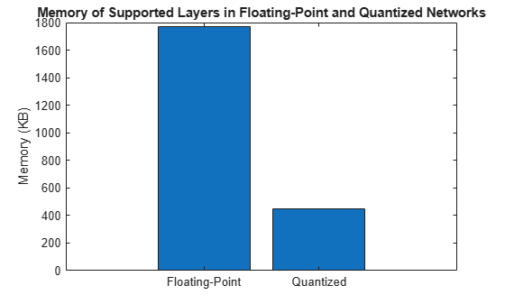
The parameter memory of the LSTM and fully connected layers in the network reduced by about 75%.
Compute the RMSE of the quantized network on the test data.
RMSEQuantized = testnet(qRecurrentNet,XVal,YVal,"rmse")RMSEQuantized = 0.0351
Compare the error of the floating-point and quantized networks
figure
bar([RMSEFloatingPoint RMSEQuantized])
xticklabels(["Floating-Point","Quantized"])
ylabel("RMSE")
title("RMSE of Floating-Point and Quantized Networks")
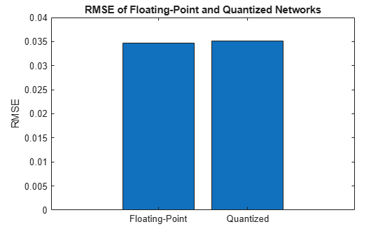
Quantizing the network has negligible impact on the RMSE of the predictions.
Simulate Quantized Network in MATLAB
The quantized network qRecurrentNet is a simulatable network. Simulate the original floating-point network and the quantized network to compare their performance to each other and to the ground truth.
Extract one sequence from the test data.
testDataPoint = 17;
xSample = XVal{:,testDataPoint};
ySample = YVal{:,testDataPoint};
17;
xSample = XVal{:,testDataPoint};
ySample = YVal{:,testDataPoint};Simulate the floating-point and quantized networks with the test data sequence.
samplePredictionFloatingPoint = predict(recurrentNet,xSample);
samplePredictionQuantized = predict(qRecurrentNet,xSample);
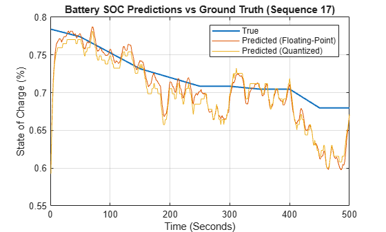
Plot the ground truth, floating-point network prediction, and quantized network prediction.
plotBSOCPrediction(ySample,samplePredictionFloatingPoint,samplePredictionQuantized,testDataPoint)
Export Quantized Network to Simulink
Export the model with quantization details to Simulink using the exportNetworkToSimulink function. This function converts the network into layer blocks. You can use layer blocks to:
Visualize the operations of each layer in a network.
Easily debug issues with a Simulink model and generated code.
Customize generated code using built-in Simulink features.
mdlInfo = exportNetworkToSimulink(qRecurrentNet, ...
    ModelName="QuantizedBSOCNetwork", ...
    ExpandNetworkSubsystem=true, ...
    Stateful=true, ...
    FrameBased=true, ...
    InputDataType="double");

To see the internal operations of each layer block, click the down arrow.
Simulate Quantized Network in Simulink
Set model parameters.
sampleTime = 1;
N = size(xSample,1);
timeSteps = (0:sampleTime:(N-1)*sampleTime)';

ts = timeseries(xSample,timeSteps,"Name",'Battery_Signals');

load_system([mdlInfo.ModelName '.slx']);

set_param(mdlInfo.ModelName,Solver="FixedStepDiscrete",FixedStep=num2str(sampleTime));
set_param(mdlInfo.ModelName,SaveOutput="on",OutputSaveName="YSimPred");
Simulate the network.
in = Simulink.SimulationInput(mdlInfo.ModelName);
in = in.setExternalInput(ts);
in = in.setModelParameter(SimulationMode="normal",StopTime=num2str(timeSteps(end)));
simOut = sim(in);
samplePredictionSimulink = simOut.YSimPred{1}.Values.Data;
Plot the ground truth, floating-point network prediction from MATLAB, and quantized network prediction from Simulink.
plotBSOCPrediction(ySample,samplePredictionFloatingPoint,samplePredictionSimulink,testDataPoint)

Generate Code
Generate and test code for the model through software-in-the-loop (SIL) simulation. Then use Embedded Coder to trace elements of the Simulink model to the generated code.
Perform Software-in-the-Loop Testing
Run SIL simulation. A SIL simulation generates source code from the model, compiles and builds the source code, and executes an application as a separate process on your host computer.
inSIL = Simulink.SimulationInput(mdlInfo.ModelName);
inSIL = inSIL.setExternalInput(ts);
inSIL = inSIL.setModelParameter(SimulationMode="software-in-the-loop",StopTime=num2str(timeSteps(end)));
simOutSIL = sim(inSIL);
Plot the ground truth, floating-point network prediction from MATLAB, and quantized network prediction from SIL.
samplePredictionSIL = simOutSIL.YSimPred{1}.Values.Data;
plotBSOCPrediction(ySample,samplePredictionFloatingPoint,samplePredictionSIL,testDataPoint)
Compare the predictions of the quantized network in Simulink and in SIL simulation.
figure
timeSteps = 1:length(ySample);
plot(timeSteps,[samplePredictionSimulink,samplePredictionSIL])
xlabel("Time (Seconds)")
ylabel("State of Charge (%)")
legend({"Predicted Simulink","Predicted SIL"}, ...
    'Location','best')
grid on
For an example of running SIL with the SIL/PIL Manager app in Simulink, see Generate Code for Battery State of Charge Estimation Using Deep Learning.
Trace Simulink Model Elements in Generated Code
Code tracing (traceability) uses hyperlinks to navigate between a line of generated code and its corresponding elements in a model. You can use this to trace which parts of the code relate to each layer.
To trace the generated code to blocks in the Simulink model:
Open the model.
Open the Embedded Coder® app. Build the model. On the C Code tab, click Build.The HTML code generation report opens by default. To use the report, see Verify Generated Code by Using Code Tracing (Embedded Coder).
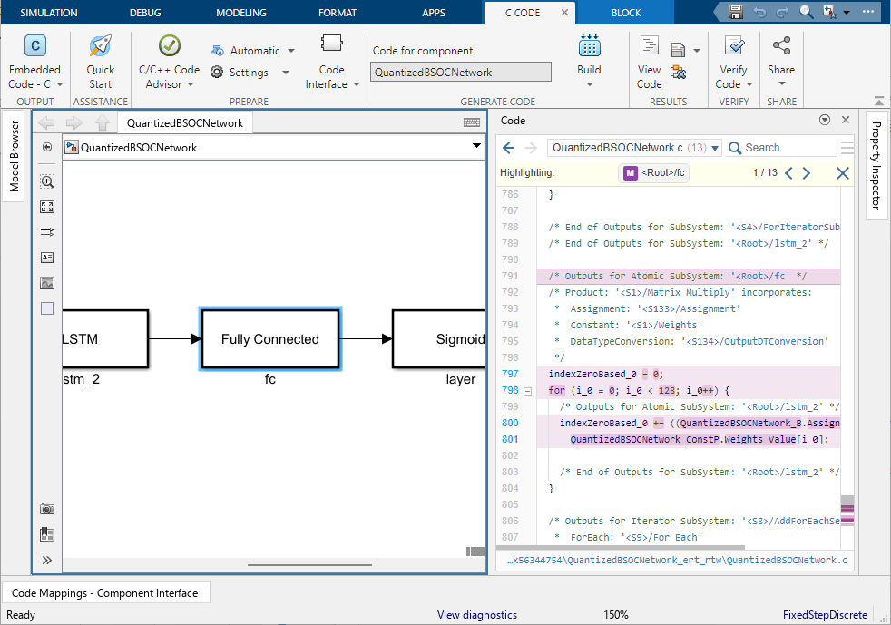
View the generated code in the Code view in the Code perspective. The source code contains traceability information such as hyperlinked comments, line numbers, variables, and operators.
In the model element, click a layer block.
In the generated code in the Code view window, you see the first instance of highlighted code that is generated for the layer block. At the top of the Code view, numbers that appear to the right of generated file names indicate the total number of highlighted lines in each file. This figure shows the result of tracing the Fully Connected Layer block in the
QuantizedBSOCNetworkmodel.
Helper Functions
Calculate Memory of Supported Layers
The estimateLayerMemory function uses the estimateNetworkMetrics function to measure the memory of each supported layer. Not all layers are supported for estimateNetworkMetrics, so the resulting number is often less than the total network memory.
function layerMemoryInKB = estimateLayerMemory(net)
    info = estimateNetworkMetrics(net);
    layerMemoryInMB = sum(info.("ParameterMemory (MB)"));
    layerMemoryInKB = layerMemoryInMB * 1000;
end
Plot Battery State of Charge Prediction
The plotBSOCPrediction function plots a comparison of the ground truth, the prediction of the floating-point network, and the prediction of the quantized network for one test sequence.
function plotBSOCPrediction(yTrue,yFloatingPoint,yQuantized,seqIdx)

% Convert data to column vectors
yTrue = squeeze(extractdata(yTrue))';
yFloatingPoint = squeeze(extractdata(yFloatingPoint))';
yQuantized = squeeze(extractdata(yQuantized))';

% Create time steps vector
timeSteps = 1:length(yTrue);

% Plot predictions
figure
plot(timeSteps,yTrue,LineWidth=1.5)
hold on
plot(timeSteps,yFloatingPoint)
plot(timeSteps,yQuantized)
hold off

xlabel("Time (Seconds)")
ylabel("State of Charge (%)")
legend({"True","Predicted (Floating-Point)","Predicted (Quantized)"}, ...
    Location="best")
title(sprintf("Battery SOC Predictions vs Ground Truth (Sequence %d)",seqIdx),FontWeight="bold")
grid on
end