HL-20 の自動操縦を調整するための MATLAB ワークフロー
これは、HL-20 機体用の飛行制御システムの設計と調整に関する例のシリーズのパート 5 です。このパートでは、Simulink® モデルを使わずに設計の大部分を MATLAB® で実行する方法を説明します。
背景
この例ではNASA HL-20 揚力体機体 (Aerospace Blockset)から応用した HL-20 モデルを使用します。詳細については、シリーズのパート 1 (HL-20 機体の平衡化と線形化) を参照してください。航空機の姿勢を制御する自動操縦には 3 つの内側のループと 3 つの外側のループが含まれます。

パート 2 (HL-20 の自動操縦における角速度の制御) およびパート 3 (HL-20 の自動操縦の姿勢制御 - SISO 設計) では、内側のループを閉じて外側のループのゲイン スケジュールを調整する方法を示しました。これらの例では slTuner インターフェイスを使用して Simulink モデルを操作し、線形化モデルと制御システム応答を取得し、調整後の値を Simulink にプッシュで戻しました。
単純なアーキテクチャと高速の設計反復を扱う場合、線形化モデルを MATLAB で操作して feedback などの基本的なコマンドを使ってループを閉じる方が好ましく、概念的にも簡単なことがあります。この例では、パート 2 と 3 の設計手順を MATLAB で実行する方法を説明します。
プラント モデルの取得
自動操縦を調整するには、偏向角から角度位置および角速度への伝達関数の線形化モデルが必要です。そのためには、"平衡化と線形化" の手順 (HL-20 機体の平衡化と線形化を参照) の結果から作業を開始します。G7 が 40 の異なる (alpha,beta) 条件における機体の 7 状態線形モデルであり、CS が Controls Selector ブロックの線形化であることを思い出してください。
load csthl20_TrimData G7 CS
I/O 選択の基準として Simulink モデル "csthl20_trim" を使用し、G7 と CS を直列に接続して目的のプラント モデルを作成します。phi、alpha、beta をラジアンから度単位に変換することを忘れないでください。
r2d = 180/pi;
G = diag([1 1 1 r2d r2d r2d]) * G7([4:7 31:32],1:6) * CS(:,1:3);

G.InputName = {'da','de','dr'};
G.OutputName = {'p','q','r','Phi_deg','Alpha_deg','Beta_deg'};

size(G)
8x5 array of state-space models. Each model has 6 outputs, 3 inputs, and 7 states.
これにより、平衡化に使用される (alpha,beta) 条件の 8 行 5 列のグリッドにわたるプラント モデルの配列が得られます。
内側のループを閉じる
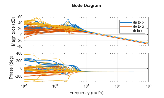
内側のループを閉じるには、パート 2 (HL-20 の自動操縦における角速度の制御) と同じ手順に従います。ゲイン Kp、Kq、Kr を選択して、p、q、r ループの交差周波数をそれぞれ 30、22.5、37.5 rad/s に設定してこれを行います。
% Compute Kp,Kq,Kr for each (alpha,beta) condition.
Gpqr = G({'p','q','r'},:);
Kp = 1./abs(evalfr(Gpqr(1,1),30i));
Kq = -1./abs(evalfr(Gpqr(2,2),22.5i));
Kr = -1./abs(evalfr(Gpqr(3,3),37.5i));

bode(Gpqr(1,1)*Kp,Gpqr(2,2)*Kq,Gpqr(3,3)*Kr,{1e-1,1e3}), grid
legend('da to p','de to q','dr to r')
feedback を使用して 3 つの内側のループを閉じます。プラント入力 da、de、dr に、後で安定余裕を評価するための解析ポイントを挿入します。
Cpqr = append(ss(Kp),ss(Kq),ss(Kr));
APu = AnalysisPoint('u',3);  APu.Location = {'da','de','dr'};

Gpos = feedback(G * APu * Cpqr, eye(3), 1:3, 1:3);
Gpos.InputName = {'p_demand','q_demand','r_demand'};

size(Gpos)
8x5 array of generalized state-space models.
Each model has 6 outputs, 3 inputs, 7 states, and 1 blocks.
これらのコマンドは、さまざまな (alpha,beta) 条件に対応するプラントとゲインの配列を扱っているという点をシームレスに管理していることに注意してください。
外側のループの調整
次に外側のループに移動します。外側のループが認識する "プラント" の線形モデルの配列 Gpos は既に取得済みです。パート 3 (HL-20 の自動操縦の姿勢制御 - SISO 設計) で行ったように、6 つのゲイン スケジュールを alpha と beta の多項式曲面としてパラメーター化します。再び比例ゲインに 2 次曲面を使用し、積分ゲインに多重線形曲面を使用します。
% Grid of (alpha,beta) design points
alpha_vec = -10:5:25;	 % Alpha Range
beta_vec = -10:5:10;     % Beta Range
[alpha,beta] = ndgrid(alpha_vec,beta_vec);
SG = struct('alpha',alpha,'beta',beta);

% Proportional gains
alphabetaBasis = polyBasis('canonical',2,2);
P_PHI = tunableSurface('Pphi', 0.05, SG, alphabetaBasis);
P_ALPHA = tunableSurface('Palpha', 0.05, SG, alphabetaBasis);
P_BETA = tunableSurface('Pbeta', -0.05, SG, alphabetaBasis);

% Integral gains
alphaBasis = @(alpha) alpha;
betaBasis = @(beta) abs(beta);
alphabetaBasis = ndBasis(alphaBasis,betaBasis);
I_PHI = tunableSurface('Iphi', 0.05, SG, alphabetaBasis);
I_ALPHA = tunableSurface('Ialpha', 0.05, SG, alphabetaBasis);
I_BETA = tunableSurface('Ibeta', -0.05, SG, alphabetaBasis);
外側のループの全体のコントローラーは 3 行 3 列の対角 PI コントローラーで、角度位置 phi、alpha、beta の誤差を受け取って速度要求 p_demand、q_demand、r_demand を計算します。
KP = append(P_PHI,P_ALPHA,P_BETA);
KI = append(I_PHI,I_ALPHA,I_BETA);
Cpos = KP + KI * tf(1,[1 0]);
最後に feedback を使用して、外側のループの調整可能な閉ループ モデルを取得します。調整と閉ループの解析を有効にするには、プラント出力に解析ポイントを挿入します。
RollOffFilter = tf(10,[1 10]);
APy = AnalysisPoint('y',3);  APy.Location = {'Phi_deg','Alpha_deg','Beta_deg'};

T0 = feedback(APy * Gpos(4:6,:) * RollOffFilter * Cpos ,eye(3));
T0.InputName = {'Phi_demand','Alpha_demand','Beta_demand'};
T0.OutputName = {'Phi_deg','Alpha_deg','Beta_deg'};
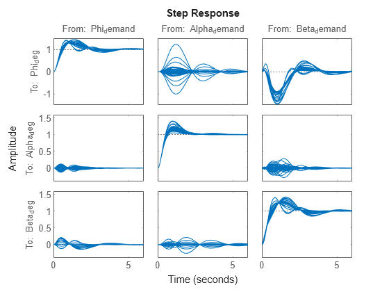
初期のゲイン曲面設定 (定数ゲイン 0.05) での閉ループ応答をプロットできます。
step(T0,6)
調整目標
パート 3 (HL-20 の自動操縦の姿勢制御 - SISO 設計) と同じ調整目標を使用します。これには外側のループのゲイン交差を 0.5 ~ 5 rad/s の間に設定する "MinLoopGain" および "MaxLoopGain" の目標が含まれます。
R1 = TuningGoal.MinLoopGain({'Phi_deg','Alpha_deg','Beta_deg'},0.5,1);
R1.LoopScaling = 'off';
R2 = TuningGoal.MaxLoopGain({'Phi_deg','Alpha_deg','Beta_deg'},tf(50,[1 10 0]));
R2.LoopScaling = 'off';
また、各ループ内およびループ間に適切な安定余裕を課す可変目標 "Margins" も含まれます。
% Gain margins vs (alpha,beta)
GM = [...
   6     6     6     6     6
   6     6     7     6     6
   7     7     7     7     7
   7     7     7     7     7
   7     7     7     7     7
   7     7     7     7     7
   6     6     7     6     6
   6     6     6     6     6];

% Phase margins vs (alpha,beta)
PM = [...
   40         40          40         40        40
   40         40          45         40        40
   45         45          45         45        45
   45         45          45         45        45
   45         45          45         45        45
   45         45          45         45        45
   40         40          45         40        40
   40         40          40         40        40];

% Create varying goal
FH = @(gm,pm) TuningGoal.Margins({'da','de','dr'},gm,pm);
R3 = varyingGoal(FH,GM,PM);
ゲイン スケジュール調整
これで、systune を使用して 6 つのゲイン曲面を 40 の設計点すべてで調整目標に対し整形できます。
T = systune(T0,[R1 R2 R3]);
Final: Soft = 1.03, Hard = -Inf, Iterations = 53
最終目的値は 1 に近いので、調整目標は実質的に満たされます。閉ループの角度応答をプロットして初期設定と比較します。
step(T0,T,6)
legend('Baseline','Tuned','Location','SouthEast')
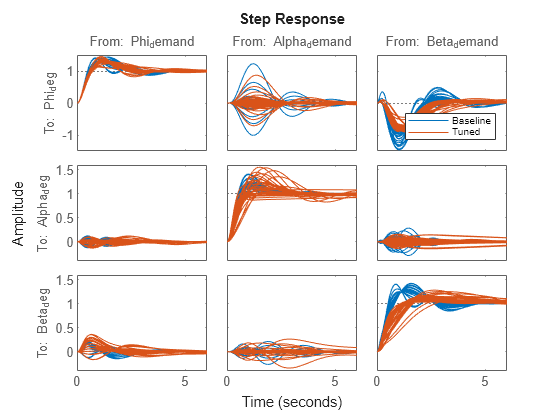
結果はパート 2 と 3 で取得したものと一致します。調整後のゲイン曲面も類似しています。
clf
% NOTE: setBlockValue updates each gain surface with the tuned coefficients in T
subplot(3,2,1), viewSurf(setBlockValue(P_PHI,T))
subplot(3,2,3), viewSurf(setBlockValue(P_ALPHA,T))
subplot(3,2,5), viewSurf(setBlockValue(P_BETA,T))
subplot(3,2,2), viewSurf(setBlockValue(I_PHI,T))
subplot(3,2,4), viewSurf(setBlockValue(I_ALPHA,T))
subplot(3,2,6), viewSurf(setBlockValue(I_BETA,T))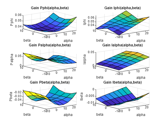
ここで、evalSurf を使用してゲイン曲面をサンプリングし、Simulink モデルのルックアップ テーブルを更新することができます。また、codegen メソッドを使ってゲイン曲面方程式のコードを生成することもできます。以下に例を示します。
% Generate code for "P phi" block
MCODE = codegen(setBlockValue(P_PHI,T));

% Get tuned values for the "I phi" lookup table
Kphi = evalSurf(setBlockValue(I_PHI,T),alpha_vec,beta_vec);