レイズド コサイン フィルター処理
この例では、レイズド コサイン フィルターの符号間干渉 (ISI) 除去力を示します。また、レイズド コサイン送信および受信フィルター System object を使用して、送信側と受信側との間でレイズド コサイン フィルター処理を分割する方法も説明します。
レイズド コサイン フィルターの仕様
レイズド コサイン フィルターの主なパラメーターは、ロールオフ係数で、これは間接的にフィルターの帯域を指定します。理想的なレイズド コサイン フィルターの実現には、タップが無限に必要となります。したがって、実際のレイズド コサイン フィルターはウィンドウ関数がかけられます。ウィンドウ長は、FilterSpanInSymbols プロパティを使用して制御されます。この例では、フィルターが 6 つのシンボル区間にまたがるため、ウィンドウ長を 6 つのシンボル区間として指定します。また、そのようなフィルターにも 3 つのシンボル区間の群遅延があります。レイズド コサイン フィルターは、信号がアップサンプリングされるパルス整形で使用されます。したがって、アップサンプリング係数を指定することも必要です。この例では、以下のパラメーターを使用してレイズド コサイン フィルターを設計します。
% Define the parameters
Nsym = 6;                                 % Filter span in symbol durations
beta = [0.1, 0.3, 0.5, 0.7, 0.9];         % Roll-off factor
sampsPerSym = 8;                          % Upsampling factor
colors = ["r", "g", "b", "c", "m"];       % Define colors for different beta values
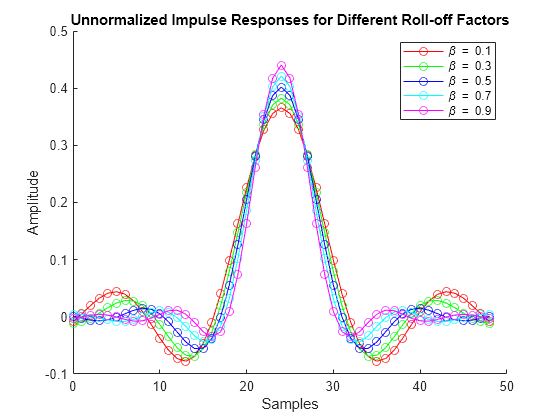
各ベータ値に対してレイズド コサイン送信フィルター System object™ を作成し、目的のフィルター特性を満たすようにそのプロパティを設定します。impz を使用してフィルター特性を可視化します。レイズド コサイン送信フィルター System object は、ユニット エネルギーで直接型ポリフェーズ FIR フィルターを設計します。フィルターには Nsym*sampsPerSym タップまたは Nsym*sampsPerSym+1 タップの次数があります。フィルター処理済みのデータとフィルター処理されていないデータが重ねられた時に一致するように、Gain プロパティを使ってフィルター係数を正規化できます。
% Create figures for plotting
figure(Name="Unnormalized Impulse Responses");
hold on;
figure(Name="Normalized Impulse Responses");
hold on;

for i = 1:length(beta)
    % Create a raised cosine transmit filter for each beta value
    rctFilt = comm.RaisedCosineTransmitFilter(RolloffFactor=beta(i), ...
        FilterSpanInSymbols=Nsym, ...
        OutputSamplesPerSymbol=sampsPerSym);

    % Extract the filter coefficients
    b = coeffs(rctFilt);

    % Compute the unnormalized impulse response
    [h_unnorm, t_unnorm] = impz(b.Numerator);

    % Switch to the unnormalized figure to plot
    figure(findobj(Name="Unnormalized Impulse Responses"));
    plot(t_unnorm, h_unnorm, colors(i), Marker="o", ...
        DisplayName=['\beta = ', num2str(beta(i))]);

    % Normalize the filter coefficients
    rctFilt.Gain = 1/max(b.Numerator);

    % Compute the normalized impulse response
    [h_norm, t_norm] = impz(b.Numerator * rctFilt.Gain);

    % Switch to the normalized figure to plot
    figure(findobj(Name="Normalized Impulse Responses"));
    plot(t_norm, h_norm, colors(i), Marker="o", ...
        DisplayName=['\beta = ', num2str(beta(i))]);
end

% The unnormalized figure
figure(findobj(Name="Unnormalized Impulse Responses"));
hold off;
title("Unnormalized Impulse Responses for Different Roll-off Factors");
xlabel("Samples");
ylabel("Amplitude");
legend("show");
figure(findobj('Name', 'Normalized Impulse Responses'));
hold off;
title("Normalized Impulse Responses for Different Roll-off Factors");
xlabel("Samples");
ylabel("Amplitude");
legend show;

レイズド コサイン フィルターを使ったパルス整形
バイポーラ データ シーケンスを生成します。さらに、レイズド コサイン フィルターを使用して、ISI を発生させずに波形を整形します。
% Parameters
DataL = 20;             % Data length in symbols
R = 1000;               % Data rate
Fs = R * sampsPerSym;   % Sampling frequency

% Create a local random stream to be used by random number generators for
% repeatability
hStr = RandStream('mt19937ar',Seed=0);

% Generate random data
x = 2*randi(hStr,[0 1],DataL,1)-1;
% Time vector sampled at symbol rate in milliseconds
tx = 1000 * (0: DataL - 1) / R;
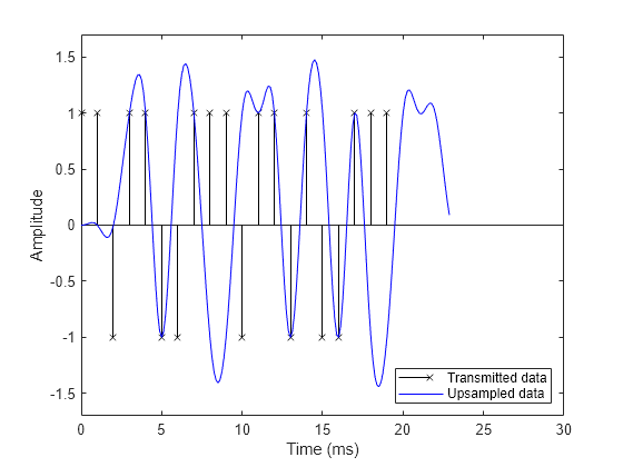
プロットでデジタル データと内挿信号を比較します。フィルターの群遅延 (Nsym/(2*R)) によりフィルターのピーク応答が遅れるため、その 2 つの信号を比較することは困難です。有益なサンプルをすべてフィルターからフラッシュするために、入力 x の末尾に Nsym/2 個のゼロを追加します。
% Design raised cosine filter with given order in symbols
rctFilt1 = comm.RaisedCosineTransmitFilter(...
  Shape='Normal', ...
  RolloffFactor=0.5, ...
  FilterSpanInSymbols=Nsym, ...
  OutputSamplesPerSymbol=sampsPerSym);


% Normalize to obtain maximum filter tap value of 1
b1 = coeffs(rctFilt1);
rctFilt1.Gain = 1/max(b1.Numerator);

% Visualize the impulse response
%impz(rctFilt.coeffs.Numerator)

% Filter
yo = rctFilt1([x; zeros(Nsym/2,1)]);
% Time vector sampled at sampling frequency in milliseconds
to = 1000 * (0: (DataL+Nsym/2)*sampsPerSym - 1) / Fs;
% Plot data
fig1 = figure;
stem(tx, x, 'kx'); hold on;
% Plot filtered data
plot(to, yo, 'b-'); hold off;
% Set axes and labels
axis([0 30 -1.7 1.7]);  xlabel('Time (ms)'); ylabel('Amplitude');
legend('Transmitted data','Upsampled data','Location','southeast')
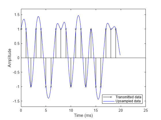
入力信号を遅らせることで、レイズド コサイン フィルターの群遅延を補正します。これで、レイズド コサイン フィルターが信号をアップサンプリングし、信号にフィルター処理を行うようすが確認しやすくなりました。フィルター処理された信号は、入力サンプル時の遅延入力信号と同一です。この結果は、ISI を回避しながらも信号を帯域制限するレイズド コサイン フィルターの機能を示しています。
% Filter group delay, since raised cosine filter is linear phase and
% symmetric.
fltDelay = Nsym / (2*R);
% Correct for propagation delay by removing filter transients
yo = yo(fltDelay*Fs+1:end);
to = 1000 * (0: DataL*sampsPerSym - 1) / Fs;
% Plot data.
stem(tx, x, 'kx'); hold on;
% Plot filtered data.
plot(to, yo, 'b-'); hold off;
% Set axes and labels.
axis([0 25 -1.7 1.7]);  xlabel('Time (ms)'); ylabel('Amplitude');
legend('Transmitted data','Upsampled data','Location','southeast')
ロールオフ係数
ロールオフ係数を 0.5 (青い曲線) から 0.2 (赤い曲線) に変更することによってフィルター処理された出力に見られる効果を示します。ロールオフ値が低いほど、フィルターの遷移帯域は狭くなります。その結果、フィルター処理済みの信号のオーバーシュートは、青い曲線より赤い曲線の方が大きくなります。
% Set roll-off factor to 0.2
rctFilt2 = comm.RaisedCosineTransmitFilter(...
  Shape='Normal', ...
  RolloffFactor=0.2, ...
  FilterSpanInSymbols=Nsym, ...
  OutputSamplesPerSymbol=sampsPerSym);
% Normalize filter
b = coeffs(rctFilt2);
rctFilt2.Gain = 1/max(b.Numerator);
% Filter
yo1 = rctFilt2([x; zeros(Nsym/2,1)]);
% Correct for propagation delay by removing filter transients
yo1 = yo1(fltDelay*Fs+1:end);
% Plot data
stem(tx, x, 'kx'); hold on;
% Plot filtered data
plot(to, yo, 'b-',to, yo1, 'r-'); hold off;
% Set axes and labels
axis([0 25 -2 2]);  xlabel('Time (ms)'); ylabel('Amplitude');
legend('Transmitted Data','beta = 0.5','beta = 0.2', ...
    'Location','southeast')

ルート レイズド コサイン フィルター
通常、レイズド コサイン フィルター処理は、送信側と受信側の間でフィルター処理を分割する際に使用されます。送信側と受信側の両方とも、ルート レイズド コサイン フィルターを採用しています。送信側のフィルターと受信側のフィルターを組み合わせたものが、レイズド コサイン フィルターです。これにより ISI は最小化されます。形状を 'Square root' として設定することによりルート レイズド コサイン フィルターを指定します。
% Design raised cosine filter with given order in symbols
rctFilt3 = comm.RaisedCosineTransmitFilter(...
  Shape="Square root", ...
  RolloffFactor=0.5, ...
  FilterSpanInSymbols=Nsym, ...
  OutputSamplesPerSymbol=sampsPerSym);
設計されたフィルターを使用し、送信側でデータのアップサンプリングとフィルター処理を行います。このプロットは、ルート レイズド コサイン フィルター使用してフィルター処理された送信信号を示します。
% Upsample and filter.
yc = rctFilt3([x; zeros(Nsym/2,1)]);
% Correct for propagation delay by removing filter transients
yc = yc(fltDelay*Fs+1:end);
% Plot data.
stem(tx, x, 'kx'); hold on;
% Plot filtered data.
plot(to, yc, 'm-'); hold off;
% Set axes and labels.
axis([0 25 -1.7 1.7]);  xlabel('Time (ms)'); ylabel('Amplitude');
legend('Transmitted data','Sqrt. raised cosine','Location','southeast')

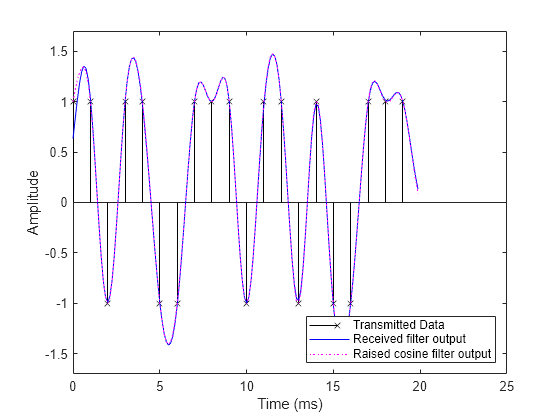
次に、送信信号 (マゼンタの曲線) を受信側でフィルター処理します (完全な波形を表示するため、フィルター出力を間引しないでください)。既定のユニット エネルギー正規化処理により、送信側フィルターと受信側フィルターの組み合わせのゲインは、正規化されたレイズド コサイン フィルターのゲインと同じになります。単一のレイズド コサイン フィルターを使用してフィルター処理された信号と結局同じとなるフィルター処理された受信信号は、受信側で青い曲線によって描かれます。
% Design and normalize filter.
rcrFilt = comm.RaisedCosineReceiveFilter(...
  'Shape',                  'Square root', ...
  'RolloffFactor',          0.5, ...
  'FilterSpanInSymbols',    Nsym, ...
  'InputSamplesPerSymbol',  sampsPerSym, ...
  'DecimationFactor',       1);
% Filter at the receiver.
yr = rcrFilt([yc; zeros(Nsym*sampsPerSym/2, 1)]);
% Correct for propagation delay by removing filter transients
yr = yr(fltDelay*Fs+1:end);
% Plot data.
stem(tx, x, 'kx'); hold on;
% Plot filtered data.
plot(to, yr, 'b-',to, yo, 'm:'); hold off;
% Set axes and labels.
axis([0 25 -1.7 1.7]);  xlabel('Time (ms)'); ylabel('Amplitude');
legend('Transmitted Data','Received filter output', ...
    'Raised cosine filter output','Location','southeast')
単一搬送波システムの PAPR に対するロールオフ係数の影響
ピーク対平均電力比 (PAPR) は、信号のピークが平均電力レベルと比較してどの程度極端であるかを定量化する尺度です。PAPR が高いということは、平均電力に比べて信号のピーク値が非常に高くなる場合があることを示しています。これは、電力増幅器にとっては問題であり、非線形歪みにつながります。
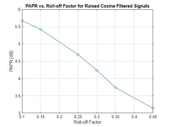
レイズド コサイン フィルターのロールオフ係数は、フィルターの通過帯域から阻止帯域までの遷移帯域幅を決定します。ロールオフ係数が低いほど遷移が急峻になり、帯域幅の使用効率は向上しますが、PAPR が高くなる可能性があります。周波数領域での遷移が急峻になると、時間領域でのピーク振幅が大きくなる可能性があります。
逆に、ロールオフ係数が高くなると、周波数領域での遷移がスムーズになり、信号の時間領域のピークが目立たなくなるため、PAPR は低くなります。ただし、この結果には帯域幅の使用量の増加という代償が伴います。
この例では、単一搬送波システムにおける 2 相位相偏移変調 (BSPK) 信号の PAPR に対するロールオフ係数の影響を示します。
N = 10000; % Number of bits
M = 2;     % Modulation order (BPSK in this case)
rolloffFactors = [0.1, 0.15, 0.25, 0.3, 0.35, 0.45];
sampsPerSym = 2;
Nsym = 6;  % Filter span in symbols

% Generate a random binary signal
data = randi([0 M-1], N, 1);

% BPSK Modulation
modData = pskmod(data, M);

% Initialize vector to store PAPR values
paprValues = zeros(length(rolloffFactors), 1);

for i = 1:length(rolloffFactors)
    % Create raised cosine transmit filter
    rctFilt = comm.RaisedCosineTransmitFilter(...
        RolloffFactor=rolloffFactors(i), ...
        FilterSpanInSymbols=Nsym, ...
        OutputSamplesPerSymbol=sampsPerSym);
    % Filter the modulated data
    txSig = rctFilt(modData);
    % Create a powermeter object for PAPR measurement
    meter = powermeter(Measurement="Peak-to-average power ratio", ...
        ComputeCCDF=true);
    % Calculate PAPR
    papr = meter(txSig);
    paprValues(i) = papr;
end

% Plot PAPR vs. roll-off factor
figure;
plot(rolloffFactors, paprValues, '-o');
xlabel("Roll-off Factor");
ylabel("PAPR (dB)");
title("PAPR vs. Roll-off Factor for Raised Cosine Filtered Signals");
grid on;
計算コスト
次の表は、ポリフェーズ FIR 内挿フィルターとポリフェーズ FIR 間引きフィルターの計算コストを比較したものです。
C1 = cost(rctFilt3);
C2 = cost(rcrFilt);
------------------------------------------------------------------------
                    Implementation Cost Comparison
------------------------------------------------------------------------
                        Multipliers  Adders  Mult/Symbol  Add/Symbol
Multirate Interpolator      49         41          49         41
Multirate Decimator         49         48           6.125      6