結果:
In the sequence of previous suggestion in Meta Cody comment for the 'My Problems' page, I also suggest to add a red alert for new comments in 'My Groups' page.
Thank you in advance.
If you use tables extensively to perform data analysis, you may at some point have wanted to add new functionalities suited to your specific applications. One straightforward idea is to create a new class that subclasses the built-in table class. You would then benefit from all inherited existing methods.
One workaround is to create a new class that wraps a table as a Property, and re-implement all the methods that you need and are already defined for table. The is not too difficult, except for the subsref method, for which I’ll provide the code below.
Class definition
Defining a wrapper of the table class is quite straightforward. In this example, I call the class “Report” because that is what I intend to use the class for, to compute and store reports. The constructor just takes a table as input:
classdef Rapport
methods
function obj = Report(t)
if isa(t, 'Report')
obj = t;
else
obj.t_ = t;
end
end
end
properties (GetAccess = private, SetAccess = private)
t_ table = table();
end
end
I designed the constructor so that it converts a table into a Report object, but also so that if we accidentally provide it with a Report object instead of a table, it will not generate an error.
Reproducing the behaviour of the table class
Implementing the existing methods of the table class for the Report class if pretty easy in most cases.
I made use of a method called “table” in order to be able to get the data back in table format instead of a Report, instead of accessing the property t_ of the object. That method can also be useful whenever you wish to use the methods or functions already existing for tables (such as writetable, rowfun, groupsummary…).
classdef Rapport
...
methods
function t = table(obj)
t = obj.t_;
end
function r = eq(obj1,obj2)
r = isequaln(table(obj1), table(obj2));
end
function ind = size(obj, varargin)
ind = size(table(obj), varargin{:});
end
function ind = height(obj, varargin)
ind = height(table(obj), varargin{:});
end
function ind = width(obj, varargin)
ind = width(table(obj), varargin{:});
end
function ind = end(A,k,n)
% ind = end(A.t_,k,n);
sz = size(table(A));
if k < n
ind = sz(k);
else
ind = prod(sz(k:end));
end
end
end
end
In the case of horzcat (same principle for vertcat), it is just a matter of converting back and forth between the table and Report classes:
classdef Rapport
...
methods
function r = horzcat(obj1,varargin)
listT = cell(1, nargin);
listT{1} = table(obj1);
for k = 1:numel(varargin)
kth = varargin{k};
if isa(kth, 'Report')
listT{k+1} = table(kth);
elseif isa(kth, 'table')
listT{k+1} = kth;
else
error('Input must be a table or a Report');
end
end
res = horzcat(listT{:});
r = Report(res);
end
end
end
Adding a new method
The plus operator already exists for the table class and works when the table contains all numeric values. It sums columns as long as the tables have the same length.
Something I think would be nice would be to be able to write t1 + t2, and that would perform an outerjoin operation between the tables and any sizes having similar indexing columns.
That would be so concise, and that's what we’re going to implement for the Report class as an example. That is called “plus operator overloading”. Of course, you could imagine that the “+” operator is used to compute something else, for example adding columns together with regard to the keys index. That depends on your needs.
Here’s a unittest example:
classdef ReportTest < matlab.unittest.TestCase
methods (Test)
function testPlusOperatorOverload(testCase)
t1 = array2table( ...
{ 'Smith', 'Male' ...
; 'JACKSON', 'Male' ...
; 'Williams', 'Female' ...
} , 'VariableNames', {'LastName' 'Gender'} ...
);
t2 = array2table( ...
{ 'Smith', 13 ...
; 'Williams', 6 ...
; 'JACKSON', 4 ...
}, 'VariableNames', {'LastName' 'Age'} ...
);
r1 = Report(t1);
r2 = Report(t2);
tRes = r1 + r2;
tExpected = Report( array2table( ...
{ 'JACKSON' , 'Male', 4 ...
; 'Smith' , 'Male', 13 ...
; 'Williams', 'Female', 6 ...
} , 'VariableNames', {'LastName' 'Gender' 'Age'} ...
) );
testCase.verifyEqual(tRes, tExpected);
end
end
end
And here’s how I’d implement the plus operator in the Report class definition, so that it also works if I add a table and a Report:
classdef Rapport
...
methods
function r = plus(obj1,obj2)
table1 = table(obj1);
table2 = table(obj2);
result = outerjoin(table1, table2 ...
, 'Type', 'full', 'MergeKeys', true);
r = reportingits.dom.Rapport(result);
end
end
end
The case of the subsref method
If we wish to access the elements of an instance the same way we would with regular tables, whether with parentheses, curly braces or directly with the name of the column, we need to implement the subsref and subsasgn methods. The second one, subsasgn is pretty easy, but subsref is a bit tricky, because we need to detect whether we’re directing towards existing methods or not.
Here’s the code:
classdef Rapport
...
methods
function A = subsasgn(A,S,B)
A.t_ = subsasgn(A.t_,S,B);
end
function B = subsref(A,S)
isTableMethod = @(m) ismember(m, methods('table'));
isReportMethod = @(m) ismember(m, methods('Report'));
switch true
case strcmp(S(1).type, '.') && isReportMethod(S(1).subs)
methodName = S(1).subs;
B = A.(methodName)(S(2).subs{:});
if numel(S) > 2
B = subsref(B, S(3:end));
end
case strcmp(S(1).type, '.') && isTableMethod (S(1).subs)
methodName = S(1).subs;
if ~isReportMethod(methodName)
error('The method "%s" needs to be implemented!', methodName)
end
otherwise
B = subsref(table(A),S(1));
if istable(B)
B = Report(B);
end
if numel(S) > 1
B = subsref(B, S(2:end));
end
end
end
end
end
Conclusion
I believe that the table class is Sealed because is case new methods are introduced in MATLAB in the future, the subclass might not be compatible if we created any or generate unexpected complexity.
The table class is a really powerful feature.
I hope this example has shown you how it is possible to extend the use of tables by adding new functionalities and maybe given you some ideas to simplify some usages. I’ve only happened to find it useful in very restricted cases, but was still happy to be able to do so.
In case you need to add other methods of the table class, you can see the list simply by calling methods(’table’).
Feel free to share your thoughts or any questions you might have! Maybe you’ll decide that doing so is a bad idea in the end and opt for another solution.
Give your LLM an easier time looking for information on mathworks.com: point it to the recently released llms.txt files. The top-level one is www.mathworks.com/llms.txt, release changes use www.mathworks.com/help/relnotes. How does it work for you??
I can't believe someone put time into this ;-)

I believe that it is very useful and important to know when we have new comments of our own problems. Although I had chosen to receive notifications about my own problems, I only receive them when I am mentioned by @.
Is it possible to add a 'New comment' alert in front of each problem on the 'My Problems' page?

The formula comes from @yuruyurau. (https://x.com/yuruyurau)
digital life 1

figure('Position',[300,50,900,900], 'Color','k');
axes(gcf, 'NextPlot','add', 'Position',[0,0,1,1], 'Color','k');
axis([0, 400, 0, 400])
SHdl = scatter([], [], 2, 'filled','o','w', 'MarkerEdgeColor','none', 'MarkerFaceAlpha',.4);
t = 0;
i = 0:2e4;
x = mod(i, 100);
y = floor(i./100);
k = x./4 - 12.5;
e = y./9 + 5;
o = vecnorm([k; e])./9;
while true
t = t + pi/90;
q = x + 99 + tan(1./k) + o.*k.*(cos(e.*9)./4 + cos(y./2)).*sin(o.*4 - t);
c = o.*e./30 - t./8;
SHdl.XData = (q.*0.7.*sin(c)) + 9.*cos(y./19 + t) + 200;
SHdl.YData = 200 + (q./2.*cos(c));
drawnow
end
digital life 2

figure('Position',[300,50,900,900], 'Color','k');
axes(gcf, 'NextPlot','add', 'Position',[0,0,1,1], 'Color','k');
axis([0, 400, 0, 400])
SHdl = scatter([], [], 2, 'filled','o','w', 'MarkerEdgeColor','none', 'MarkerFaceAlpha',.4);
t = 0;
i = 0:1e4;
x = i;
y = i./235;
e = y./8 - 13;
while true
t = t + pi/240;
k = (4 + sin(y.*2 - t).*3).*cos(x./29);
d = vecnorm([k; e]);
q = 3.*sin(k.*2) + 0.3./k + sin(y./25).*k.*(9 + 4.*sin(e.*9 - d.*3 + t.*2));
SHdl.XData = q + 30.*cos(d - t) + 200;
SHdl.YData = 620 - q.*sin(d - t) - d.*39;
drawnow
end
digital life 3

figure('Position',[300,50,900,900], 'Color','k');
axes(gcf, 'NextPlot','add', 'Position',[0,0,1,1], 'Color','k');
axis([0, 400, 0, 400])
SHdl = scatter([], [], 1, 'filled','o','w', 'MarkerEdgeColor','none', 'MarkerFaceAlpha',.4);
t = 0;
i = 0:1e4;
x = mod(i, 200);
y = i./43;
k = 5.*cos(x./14).*cos(y./30);
e = y./8 - 13;
d = (k.^2 + e.^2)./59 + 4;
a = atan2(k, e);
while true
t = t + pi/20;
q = 60 - 3.*sin(a.*e) + k.*(3 + 4./d.*sin(d.^2 - t.*2));
c = d./2 + e./99 - t./18;
SHdl.XData = q.*sin(c) + 200;
SHdl.YData = (q + d.*9).*cos(c) + 200;
drawnow; pause(1e-2)
end
digital life 4

figure('Position',[300,50,900,900], 'Color','k');
axes(gcf, 'NextPlot','add', 'Position',[0,0,1,1], 'Color','k');
axis([0, 400, 0, 400])
SHdl = scatter([], [], 1, 'filled','o','w', 'MarkerEdgeColor','none', 'MarkerFaceAlpha',.4);
t = 0;
i = 0:4e4;
x = mod(i, 200);
y = i./200;
k = x./8 - 12.5;
e = y./8 - 12.5;
o = (k.^2 + e.^2)./169;
d = .5 + 5.*cos(o);
while true
t = t + pi/120;
SHdl.XData = x + d.*k.*sin(d.*2 + o + t) + e.*cos(e + t) + 100;
SHdl.YData = y./4 - o.*135 + d.*6.*cos(d.*3 + o.*9 + t) + 275;
SHdl.CData = ((d.*sin(k).*sin(t.*4 + e)).^2).'.*[1,1,1];
drawnow;
end
digital life 5

figure('Position',[300,50,900,900], 'Color','k');
axes(gcf, 'NextPlot','add', 'Position',[0,0,1,1], 'Color','k');
axis([0, 400, 0, 400])
SHdl = scatter([], [], 1, 'filled','o','w',...
'MarkerEdgeColor','none', 'MarkerFaceAlpha',.4);
t = 0;
i = 0:1e4;
x = mod(i, 200);
y = i./55;
k = 9.*cos(x./8);
e = y./8 - 12.5;
while true
t = t + pi/120;
d = (k.^2 + e.^2)./99 + sin(t)./6 + .5;
q = 99 - e.*sin(atan2(k, e).*7)./d + k.*(3 + cos(d.^2 - t).*2);
c = d./2 + e./69 - t./16;
SHdl.XData = q.*sin(c) + 200;
SHdl.YData = (q + 19.*d).*cos(c) + 200;
drawnow;
end
digital life 6

clc; clear
figure('Position',[300,50,900,900], 'Color','k');
axes(gcf, 'NextPlot','add', 'Position',[0,0,1,1], 'Color','k');
axis([0, 400, 0, 400])
SHdl = scatter([], [], 2, 'filled','o','w', 'MarkerEdgeColor','none', 'MarkerFaceAlpha',.4);
t = 0;
i = 1:1e4;
y = i./790;
k = y; idx = y < 5;
k(idx) = 6 + sin(bitxor(floor(y(idx)), 1)).*6;
k(~idx) = 4 + cos(y(~idx));
while true
t = t + pi/90;
d = sqrt((k.*cos(i + t./4)).^2 + (y/3-13).^2);
q = y.*k.*cos(i + t./4)./5.*(2 + sin(d.*2 + y - t.*4));
c = d./3 - t./2 + mod(i, 2);
SHdl.XData = q + 90.*cos(c) + 200;
SHdl.YData = 400 - (q.*sin(c) + d.*29 - 170);
drawnow; pause(1e-2)
end
digital life 7

clc; clear
figure('Position',[300,50,900,900], 'Color','k');
axes(gcf, 'NextPlot','add', 'Position',[0,0,1,1], 'Color','k');
axis([0, 400, 0, 400])
SHdl = scatter([], [], 2, 'filled','o','w', 'MarkerEdgeColor','none', 'MarkerFaceAlpha',.4);
t = 0;
i = 1:1e4;
y = i./345;
x = y; idx = y < 11;
x(idx) = 6 + sin(bitxor(floor(x(idx)), 8))*6;
x(~idx) = x(~idx)./5 + cos(x(~idx)./2);
e = y./7 - 13;
while true
t = t + pi/120;
k = x.*cos(i - t./4);
d = sqrt(k.^2 + e.^2) + sin(e./4 + t)./2;
q = y.*k./d.*(3 + sin(d.*2 + y./2 - t.*4));
c = d./2 + 1 - t./2;
SHdl.XData = q + 60.*cos(c) + 200;
SHdl.YData = 400 - (q.*sin(c) + d.*29 - 170);
drawnow; pause(5e-3)
end
digital life 8

clc; clear
figure('Position',[300,50,900,900], 'Color','k');
axes(gcf, 'NextPlot','add', 'Position',[0,0,1,1], 'Color','k');
axis([0, 400, 0, 400])
SHdl{6} = [];
for j = 1:6
SHdl{j} = scatter([], [], 2, 'filled','o','w', 'MarkerEdgeColor','none', 'MarkerFaceAlpha',.3);
end
t = 0;
i = 1:2e4;
k = mod(i, 25) - 12;
e = i./800; m = 200;
theta = pi/3;
R = [cos(theta) -sin(theta); sin(theta) cos(theta)];
while true
t = t + pi/240;
d = 7.*cos(sqrt(k.^2 + e.^2)./3 + t./2);
XY = [k.*4 + d.*k.*sin(d + e./9 + t);
e.*2 - d.*9 - d.*9.*cos(d + t)];
for j = 1:6
XY = R*XY;
SHdl{j}.XData = XY(1,:) + m;
SHdl{j}.YData = XY(2,:) + m;
end
drawnow;
end
digital life 9

clc; clear
figure('Position',[300,50,900,900], 'Color','k');
axes(gcf, 'NextPlot','add', 'Position',[0,0,1,1], 'Color','k');
axis([0, 400, 0, 400])
SHdl{14} = [];
for j = 1:14
SHdl{j} = scatter([], [], 2, 'filled','o','w', 'MarkerEdgeColor','none', 'MarkerFaceAlpha',.1);
end
t = 0;
i = 1:2e4;
k = mod(i, 50) - 25;
e = i./1100; m = 200;
theta = pi/7;
R = [cos(theta) -sin(theta); sin(theta) cos(theta)];
while true
t = t + pi/240;
d = 5.*cos(sqrt(k.^2 + e.^2) - t + mod(i, 2));
XY = [k + k.*d./6.*sin(d + e./3 + t);
90 + e.*d - e./d.*2.*cos(d + t)];
for j = 1:14
XY = R*XY;
SHdl{j}.XData = XY(1,:) + m;
SHdl{j}.YData = XY(2,:) + m;
end
drawnow;
end
In https://www.mathworks.com/matlabcentral/answers/38165-how-to-remove-decimal#comment_3345149 @Luisa asks,
@Cody Team, how can I vote or give a like in great comments?
It seems that there are not such options.

It’s exciting to dive into a new dataset full of unfamiliar variables but it can also be overwhelming if you’re not sure where to start. Recently, I discovered some new interactive features in MATLAB live scripts that make it much easier to get an overview of your data. With just a few clicks, you can display sparklines and summary statistics using table variables, sort and filter variables, and even have MATLAB generate the corresponding code for reproducibility.
The Graphics and App Building blog published an article that walks through these features showing how to explore, clean, and analyze data—all without writing any code.
If you’re interested in streamlining your exploratory data analysis or want to see what’s new in live scripts, you might find it helpful:
If you’ve tried these features or have your own tips for quick data exploration in MATLAB, I’d love to hear your thoughts!
Pure Matlab
82%
Simulink
18%
11 票
If you have solved a Cody problem before, you have likely seen the Scratch Pad text field below the Solution text field. It provides a quick way to get feedback on your solution before submitting it. Since submitting a solution takes you to a new page, any time a wrong solution is submitted, you have to navigate back to the problem page to try it again.
Instead, I use the Scratch Pad to test my solution repeatedly before submitting. That way, I get to a working solution faster without having to potentially go back and forth many times between the problem page and the wrong-solution page.
Here is my approach:
- Write a tentative solution.
- Copy a test case from the test suite into the Scratch Pad.
- Click the Run Function button—this is immediately below the Scratch Pad and above the Output panel and Submit buttons.
- If the solution does not work, modify the solution code, sometimes putting in disp() lines and/or removing semicolons to trace what the code is doing. Repeat until the solution passes.
- If the solution does work, repeat steps 2 through 4.
- Once there are no more test cases to copy and paste, clean up the code, if necessary (delete disp lines, reinstate all semicolons to suppress output). Click the Run Function button once more, just to make sure I did not break the solution while cleaning it up. Then, click the Submit button.
For problems with large test suites, you may find it useful to copy and paste in multiple test cases per iteration.
Hopefully you find this useful.
Jorge Bernal-AlvizJorge Bernal-Alviz shared the following code that requires R2025a or later:
Test()

function Test()
duration = 10;
numFrames = 800;
frameInterval = duration / numFrames;
w = 400;
t = 0;
i_vals = 1:10000;
x_vals = i_vals;
y_vals = i_vals / 235;
r = linspace(0, 1, 300)';
g = linspace(0, 0.1, 300)';
b = linspace(1, 0, 300)';
r = r * 0.8 + 0.1;
g = g * 0.6 + 0.1;
b = b * 0.9 + 0.1;
customColormap = [r, g, b];
figure('Position', [100, 100, w, w], 'Color', [0, 0, 0]);
axis equal;
axis off;
xlim([0, w]);
ylim([0, w]);
hold on;
colormap default;
colormap(customColormap);
plothandle = scatter([], [], 1, 'filled', 'MarkerFaceAlpha', 0.12);
for i = 1:numFrames
t = t + pi/240;
k = (4 + 3 * sin(y_vals * 2 - t)) .* cos(x_vals / 29);
e = y_vals / 8 - 13;
d = sqrt(k.^2 + e.^2);
c = d - t;
q = 3 * sin(2 * k) + 0.3 ./ (k + 1e-10) + ...
sin(y_vals / 25) .* k .* (9 + 4 * sin(9 * e - 3 * d + 2 * t));
points_x = q + 30 * cos(c) + 200;
points_y = q .* sin(c) + 39 * d - 220;
points_y = w - points_y;
CData = (1 + sin(0.1 * (d - t))) / 3;
CData = max(0, min(1, CData));
set(plothandle, 'XData', points_x, 'YData', points_y, 'CData', CData);
brightness = 0.5 + 0.3 * sin(t * 0.2);
set(plothandle, 'MarkerFaceAlpha', brightness);
drawnow;
pause(frameInterval);
end
end
Pick a team, solve Cody problems, and share your best tips and tricks. Whether you’re a beginner or a seasoned MATLAB user, you’ll have fun learning, connecting with others, and competing for amazing prizes, including MathWorks swags, Amazon gift cards, and virtual badges.
How to Participate
- Join a team that matches your coding personality
- Solve Cody problems, complete the contest problem group, or share Tips & Tricks articles
- Bonus Round: Two top players from each team will be invited to a fun code-along event
Contest Timeline
- Main Round: Nov 10 – Dec 7, 2025
- Bonus Round: Dec 8 – Dec 19, 2025
Prizes (updated 11/19)
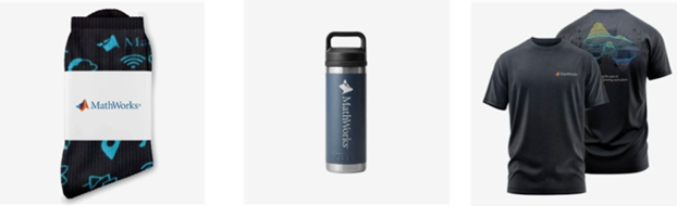
- (New prize) Solving just one problem in the contest problem group gives you a chance to win MathWorks T-shirts or socks each week.
- Finishing the entire problem group will greatly increase your chances—while helping your team win.
- Share high-quality Tips & Tricks articles to earn you a coveted MathWorks Yeti Bottle.
- Become a top finisher in your team to win Amazon gift cards and an invitation to the bonus round.
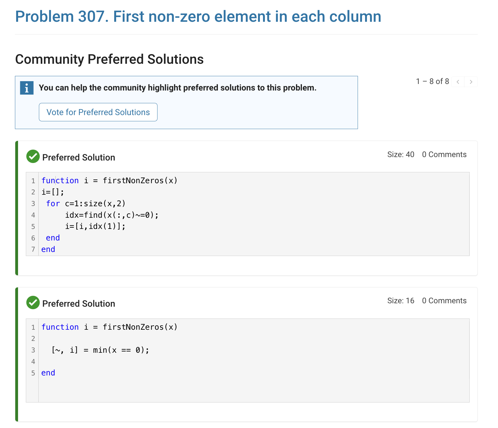
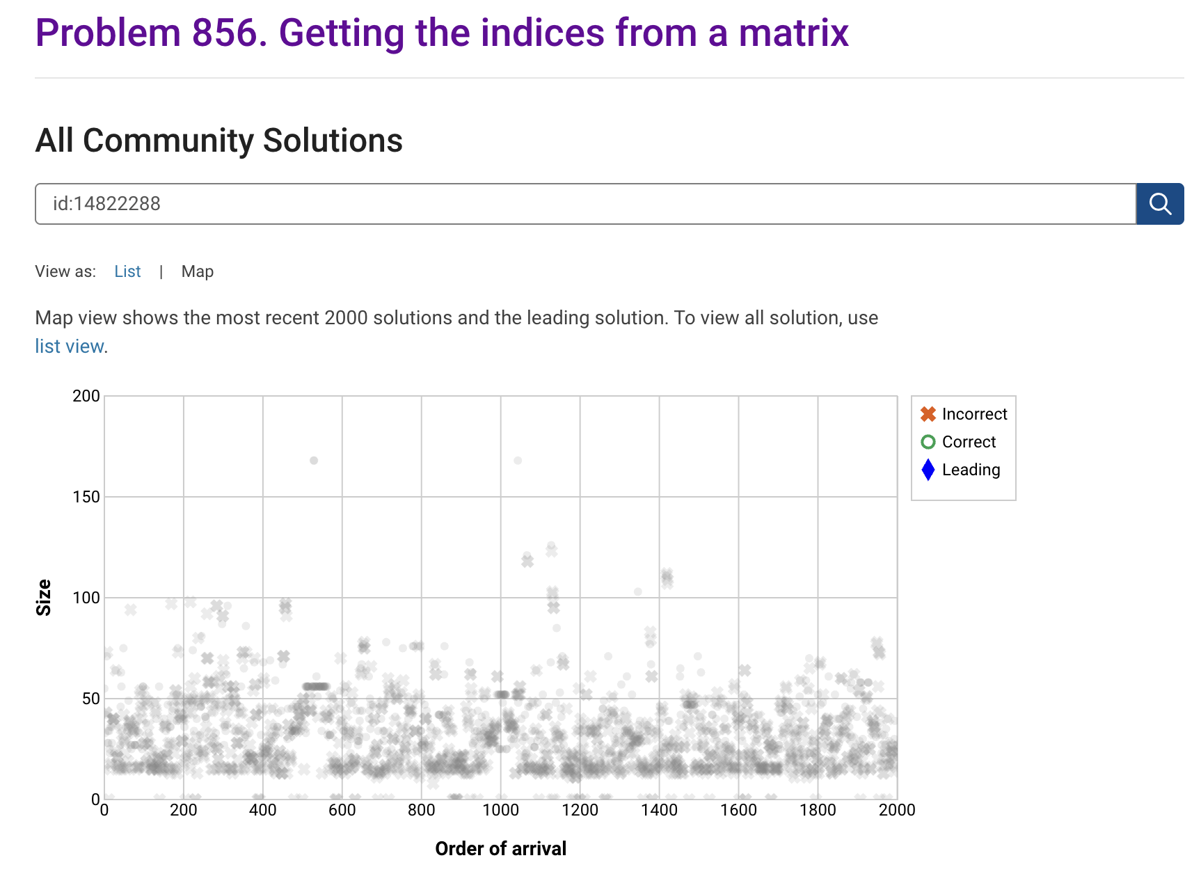
The all-community-solutions view shows the ID of each solution, and you can click on the link to go to the solution.
The preferred-community-solutions view does not show the solution IDs and does not link to the solutions. As far as I can tell, there is no way to get from that view to the solutions. If, for example, you want to go to the solution to leave a comment there, you can't.
All-community-solutions view:
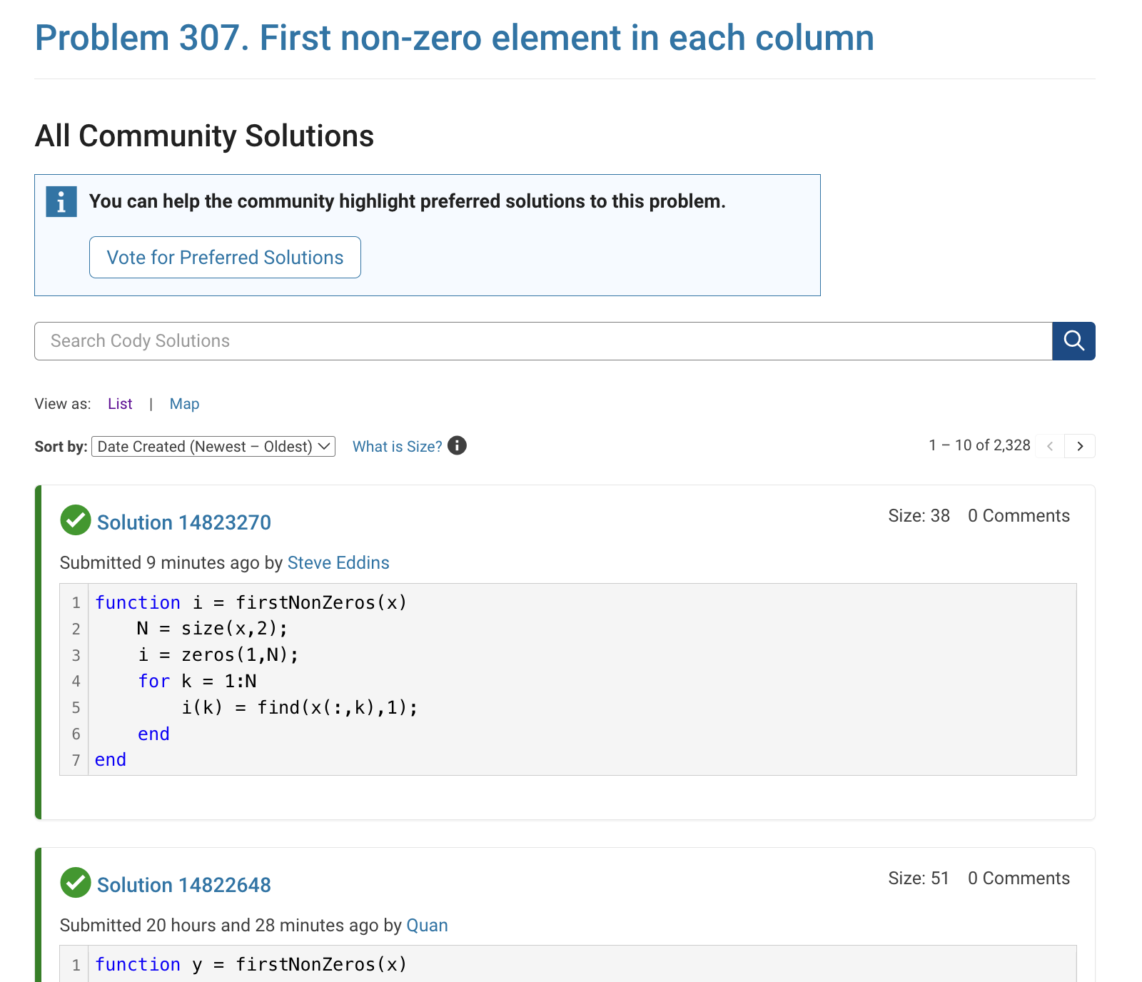
Preferred-community-solutions view, with no solution IDs and no links:
Hi cody fellows,
I already solved more than 500 problems -months ago, last july if I remember well- and get this scholar badge, but then it suddenly disappeared a few weeks later. I then solved a few more problems and it reappeared.
Now I observed it disappeared once more a few days ago.
Have you also noticed this erratic behavior of the scholar badge ? Is it normal and / or intentional ? If not, how to explain it ? (deleted problems ?)
Cheers,
Nicolas
I'm seeing solution maps shown with low-contrast gray colors instead of the correct symbol colors. I have observed this using both Safari and Chrome. Screenshot:
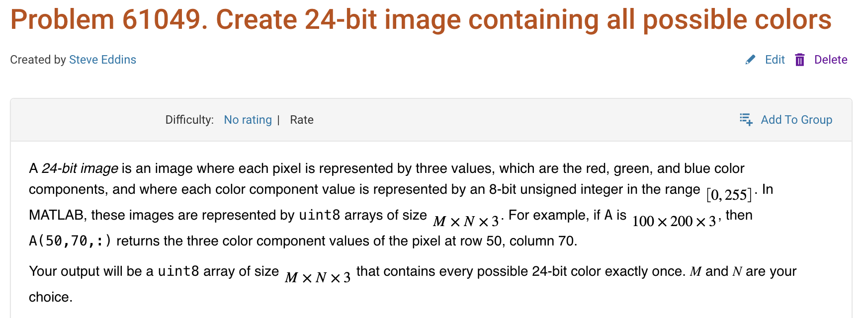
Here is a screenshot of a Cody problem that I just created. The math rendering is poor. (I have since edited the problem to remove the math formatting.)
I just learned you can access MATLAB Online from the following shortcut in your web browser: https://matlab.new
Thanks @Yann Debray
From his recent blog post: pip & uv in MATLAB Online » Artificial Intelligence - MATLAB & Simulink
Are there any code restrictions for programming Cody solutions? I could not find anything mentioned at https://www.mathworks.com/matlabcentral/content/cody/about.html, other than toolbox functions not being available.
Inspired by @xingxingcui's post about old MATLAB versions and @유장's post about an old Easter egg, I thought it might be fun to share some MATLAB-Old-Timer Stories™.
Back in the early 90s, MATLAB had been ported to MacOS, but there were some interesting wrinkles. One that kept me earning my money as a computer lab tutor was that MATLAB required file names to follow Windows standards - no spaces or other special characters. But on a Mac, nothing stopped you from naming your script "hello world - 123.m". The problem came when you tried to run it. MATLAB was essentially doing an eval on the script name, assuming the file name would follow Windows (and MATLAB) naming rules.
So now imagine a lab full of students taking a university course. As is common in many universities, the course was given a numeric code. For whatever historical reason, my school at that time was also using numeric codes for the departments. Despite being told the rules for naming scripts, many students would default to something like "26.165 - 1.1" for problem one on HW1 for the intro applied math course 26.165.
No matter what they did in their script, when they ran it, MATLAB would just say "ans = 25.0650".
Nothing brings you more MATLAB-god credibility as a student tutor than walking over to someone's computer, taking one look at their output, saying "rename your file", and walking away like a boss.
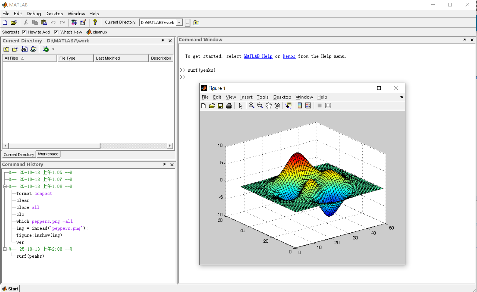
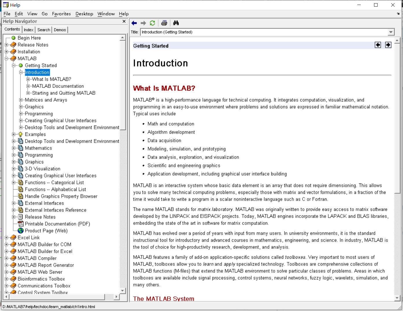
It was 2010 when I was a sophomore in university. I chose to learn MATLAB because of a mathematical modeling competition, and the university provided MATLAB 7.0, a very classic release. To get started, I borrowed many MATLAB books from the library and began by learning simple numerical calculations, plotting, and solving equations. Gradually I was drawn in by MATLAB’s powerful capabilities and became interested; I often used it as a big calculator for fun. That version didn’t have MATLAB Live Script; instead it used MATLAB Notebook (M-Book), which allowed MATLAB functions to be used directly within Microsoft Word, and it also had the Symbolic Math Toolbox’s MuPAD interactive environment. These were later gradually replaced by Live Scripts introduced in R2016a. There are many similar examples...
Out of curiosity, I still have screenshots on my computer showing MATLAB 7.0 running compatibly. I’d love to hear your thoughts?