結果:
The Ans Hack is a dubious way to shave a few points off your solution score. Instead of a standard answer like this
function y = times_two(x)
y = 2*x;
end
you would do this
function ans = times_two(x)
2*x;
end
The ans variable is automatically created when there is no left-hand side to an evaluated expression. But it makes for an ugly function. I don't think anyone actually defends it as a good practice. The question I would ask is: is it so offensive that it should be specifically disallowed by the rules? Or is it just one of many little hacks that you see in Cody, inelegant but tolerable in the context of the surrounding game?
Incidentally, I wrote about the Ans Hack long ago on the Community Blog. Dealing with user-unfriendly code is also one of the reasons we created the Head-to-Head voting feature. Some techniques are good for your score, and some are good for your code readability. You get to decide with you care about.
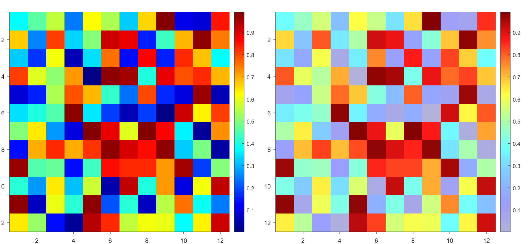
Many times when ploting, we not only need to set the color of the plot, but also its
transparency, Then how we set the alphaData of colorbar at the same time ?
It seems easy to do so :
data = rand(12,12);
% Transparency range 0-1, .3-1 for better appearance here
AData = rescale(- data, .3, 1);
% Draw an imagesc with numerical control over colormap and transparency
imagesc(data, 'AlphaData',AData);
colormap(jet);
ax = gca;
ax.DataAspectRatio = [1,1,1];
ax.TickDir = 'out';
ax.Box = 'off';
% get colorbar object
CBarHdl = colorbar;
pause(1e-16)
% Modify the transparency of the colorbar
CData = CBarHdl.Face.Texture.CData;
ALim = [min(min(AData)), max(max(AData))];
CData(4,:) = uint8(255.*rescale(1:size(CData, 2), ALim(1), ALim(2)));
CBarHdl.Face.Texture.ColorType = 'TrueColorAlpha';
CBarHdl.Face.Texture.CData = CData;
But !!!!!!!!!!!!!!! We cannot preserve the changes when saving them as images :
It seems that when saving plots, the `Texture` will be refresh, but the `Face` will not :
however, object Face only have 4 colors to change(The four corners of a quadrilateral), how
can we set more colors ??
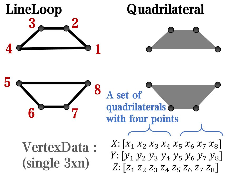
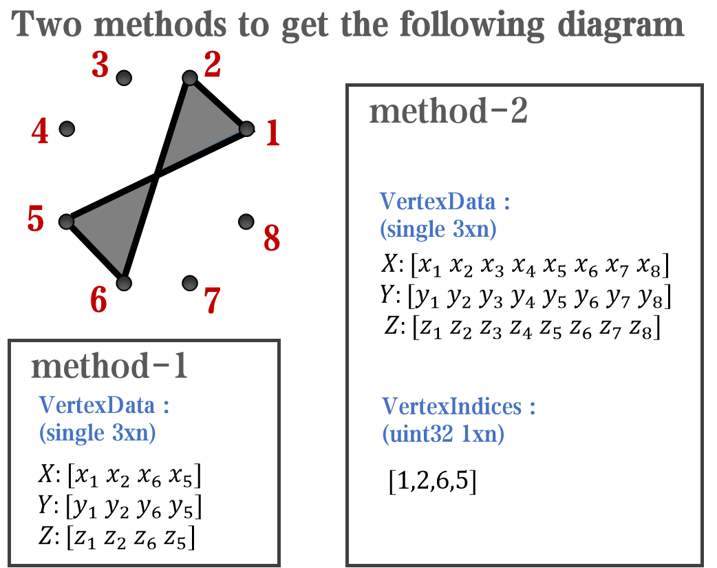
`Face` is a quadrilateral object, and we can change the `VertexData` to draw more than one little quadrilaterals:
data = rand(12,12);
% Transparency range 0-1, .3-1 for better appearance here
AData = rescale(- data, .3, 1);
%Draw an imagesc with numerical control over colormap and transparency
imagesc(data, 'AlphaData',AData);
colormap(jet);
ax = gca;
ax.DataAspectRatio = [1,1,1];
ax.TickDir = 'out';
ax.Box = 'off';
% get colorbar object
CBarHdl = colorbar;
pause(1e-16)
% Modify the transparency of the colorbar
CData = CBarHdl.Face.Texture.CData;
ALim = [min(min(AData)), max(max(AData))];
CData(4,:) = uint8(255.*rescale(1:size(CData, 2), ALim(1), ALim(2)));
warning off
CBarHdl.Face.ColorType = 'TrueColorAlpha';
VertexData = CBarHdl.Face.VertexData;
tY = repmat((1:size(CData,2))./size(CData,2), [4,1]);
tY1 = tY(:).'; tY2 = tY - tY(1,1); tY2(3:4,:) = 0; tY2 = tY2(:).';
tM1 = [tY1.*0 + 1; tY1; tY1.*0 + 1];
tM2 = [tY1.*0; tY2; tY1.*0];
CBarHdl.Face.VertexData = repmat(VertexData, [1,size(CData,2)]).*tM1 + tM2;
CBarHdl.Face.ColorData = reshape(repmat(CData, [4,1]), 4, []);
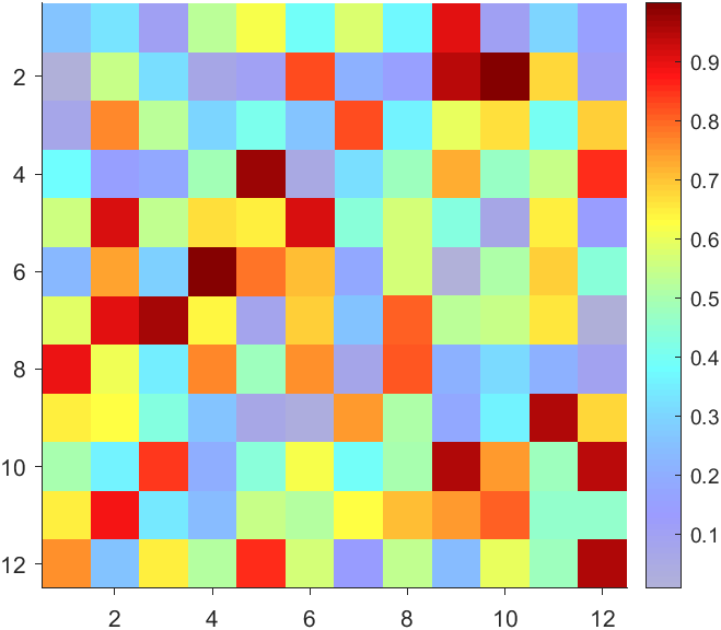
The higher the value, the more transparent it becomes
data = rand(12,12);
AData = rescale(- data, .3, 1);
imagesc(data, 'AlphaData',AData);
colormap(jet);
ax = gca;
ax.DataAspectRatio = [1,1,1];
ax.TickDir = 'out';
ax.Box = 'off';
CBarHdl = colorbar;
pause(1e-16)
CData = CBarHdl.Face.Texture.CData;
ALim = [min(min(AData)), max(max(AData))];
CData(4,:) = uint8(255.*rescale(size(CData, 2):-1:1, ALim(1), ALim(2)));
warning off
CBarHdl.Face.ColorType = 'TrueColorAlpha';
VertexData = CBarHdl.Face.VertexData;
tY = repmat((1:size(CData,2))./size(CData,2), [4,1]);
tY1 = tY(:).'; tY2 = tY - tY(1,1); tY2(3:4,:) = 0; tY2 = tY2(:).';
tM1 = [tY1.*0 + 1; tY1; tY1.*0 + 1];
tM2 = [tY1.*0; tY2; tY1.*0];
CBarHdl.Face.VertexData = repmat(VertexData, [1,size(CData,2)]).*tM1 + tM2;
CBarHdl.Face.ColorData = reshape(repmat(CData, [4,1]), 4, []);
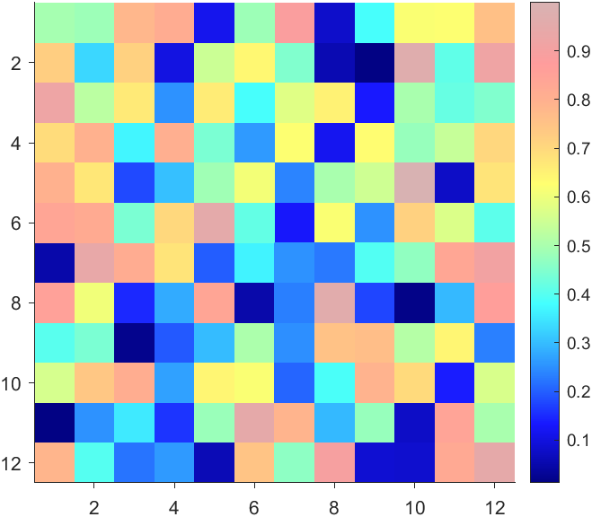
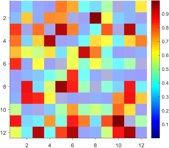
More transparent in the middle
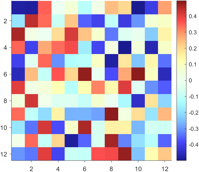
data = rand(12,12) - .5;
AData = rescale(abs(data), .1, .9);
imagesc(data, 'AlphaData',AData);
colormap(jet);
ax = gca;
ax.DataAspectRatio = [1,1,1];
ax.TickDir = 'out';
ax.Box = 'off';
CBarHdl = colorbar;
pause(1e-16)
CData = CBarHdl.Face.Texture.CData;
ALim = [min(min(AData)), max(max(AData))];
CData(4,:) = uint8(255.*rescale(abs((1:size(CData, 2)) - (1 + size(CData, 2))/2), ALim(1), ALim(2)));
warning off
CBarHdl.Face.ColorType = 'TrueColorAlpha';
VertexData = CBarHdl.Face.VertexData;
tY = repmat((1:size(CData,2))./size(CData,2), [4,1]);
tY1 = tY(:).'; tY2 = tY - tY(1,1); tY2(3:4,:) = 0; tY2 = tY2(:).';
tM1 = [tY1.*0 + 1; tY1; tY1.*0 + 1];
tM2 = [tY1.*0; tY2; tY1.*0];
CBarHdl.Face.VertexData = repmat(VertexData, [1,size(CData,2)]).*tM1 + tM2;
CBarHdl.Face.ColorData = reshape(repmat(CData, [4,1]), 4, []);
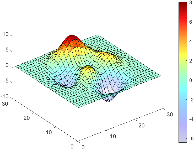
The code will work if the plot have AlphaData property
data = peaks(30);
AData = rescale(data, .2, 1);
surface(data, 'FaceAlpha','flat','AlphaData',AData);
colormap(jet(100));
ax = gca;
ax.DataAspectRatio = [1,1,1];
ax.TickDir = 'out';
ax.Box = 'off';
view(3)
CBarHdl = colorbar;
pause(1e-16)
CData = CBarHdl.Face.Texture.CData;
ALim = [min(min(AData)), max(max(AData))];
CData(4,:) = uint8(255.*rescale(1:size(CData, 2), ALim(1), ALim(2)));
warning off
CBarHdl.Face.ColorType = 'TrueColorAlpha';
VertexData = CBarHdl.Face.VertexData;
tY = repmat((1:size(CData,2))./size(CData,2), [4,1]);
tY1 = tY(:).'; tY2 = tY - tY(1,1); tY2(3:4,:) = 0; tY2 = tY2(:).';
tM1 = [tY1.*0 + 1; tY1; tY1.*0 + 1];
tM2 = [tY1.*0; tY2; tY1.*0];
CBarHdl.Face.VertexData = repmat(VertexData, [1,size(CData,2)]).*tM1 + tM2;
CBarHdl.Face.ColorData = reshape(repmat(CData, [4,1]), 4, []);

While searching the internet for some books on ordinary differential equations, I came across a link that I believe is very useful for all math students and not only. If you are interested in ODEs, it's worth taking the time to study it.
A First Look at Ordinary Differential Equations by Timothy S. Judson is an excellent resource for anyone looking to understand ODEs better. Here's a brief overview of the main topics covered:
- Introduction to ODEs: Basic concepts, definitions, and initial differential equations.
- Methods of Solution:
- Separable equations
- First-order linear equations
- Exact equations
- Transcendental functions
- Applications of ODEs: Practical examples and applications in various scientific fields.
- Systems of ODEs: Analysis and solutions of systems of differential equations.
- Series and Numerical Methods: Use of series and numerical methods for solving ODEs.
This book provides a clear and comprehensive introduction to ODEs, making it suitable for students and new researchers in mathematics. If you're interested, you can explore the book in more detail here: A First Look at Ordinary Differential Equations.
. I am using MATLAB R2023b and learning simulink and facing dificulty in finding the run button. Any solution Please.
Your kind help will be appreciated
There are a host of problems on Cody that require manipulation of the digits of a number. Examples include summing the digits of a number, separating the number into its powers, and adding very large numbers together.
If you haven't come across this trick yet, you might want to write it down (or save it electronically):
digits = num2str(4207) - '0'
That code results in the following:
digits =
4 2 0 7
Now, summing the digits of the number is easy:
sum(digits)
ans =
13
Hello and a warm welcome to everyone! We're excited to have you in the Cody Discussion Channel. To ensure the best possible experience for everyone, it's important to understand the types of content that are most suitable for this channel.
Content that belongs in the Cody Discussion Channel:
- Tips & tricks: Discuss strategies for solving Cody problems that you've found effective.
- Ideas or suggestions for improvement: Have thoughts on how to make Cody better? We'd love to hear them.
- Issues: Encountering difficulties or bugs with Cody? Let us know so we can address them.
- Requests for guidance: Stuck on a Cody problem? Ask for advice or hints, but make sure to show your efforts in attempting to solve the problem first.
- General discussions: Anything else related to Cody that doesn't fit into the above categories.
Content that does not belong in the Cody Discussion Channel:
- Comments on specific Cody problems: Examples include unclear problem descriptions or incorrect testing suites.
- Comments on specific Cody solutions: For example, you find a solution creative or helpful.
Please direct such comments to the Comments section on the problem or solution page itself.
We hope the Cody discussion channel becomes a vibrant space for sharing expertise, learning new skills, and connecting with others.
It is necessary to find a solution that satisfies the boundary conditions:
u′′′+u′+λu=f.
initial conditions:
u′′(0)= u′(0)+
 u(0),
u(0),
u′′(1)= u(1),
u(1),
u′(1)= u(1),
u(1),
How to define u and fin matlab?
where λ>0, 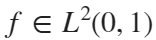 ;
; ,
,  ,
,  and
and  - given numbers.
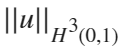 ≤
≤ where C is a positive constant independent of 𝑢 and f
clear;
syms y(x) y0 lambda u
Dy = diff(y);
D2y = diff(y,2);
D2y_2 = diff(y,2);
D3y = diff(y,3);
ode = D3y + lambda*u == y(x);
ySol(x) = dsolve(ode);
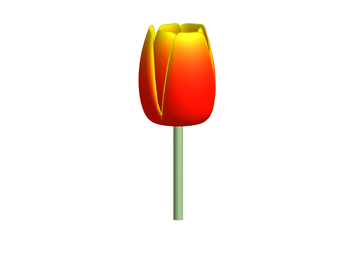
Spring is here in Natick and the tulips are blooming! While tulips appear only briefly here in Massachusetts, they provide a lot of bright and diverse colors and shapes. To celebrate this cheerful flower, here's some code to create your own tulip!
How to leave feedback on a doc page
Leaving feedback is a two-step process. At the bottom of most pages in the MATLAB documentation is a star rating.
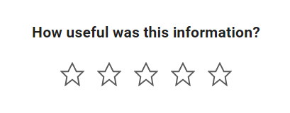
Start by selecting a star that best answers the question. After selecting a star rating, an edit box appears where you can offer specific feedback.
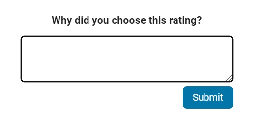
When you press "Submit" you'll see the confirmation dialog below. You cannot go back and edit your content, although you can refresh the page to go through that process again.

Tips on leaving feedback
- Be productive. The reader should clearly understand what action you'd like to see, what was unclear, what you think needs work, or what areas were really helpful.
- Positive feedback is also helpful. By nature, feedback often focuses on suggestions for changes but it also helps to know what was clear and what worked well.
- Point to specific areas of the page. This helps the reader to narrow the focus of the page to the area described by your feedback.
What happens to that feedback?
Before working at MathWorks I often left feedback on documentation pages but I never knew what happens after that. One day in 2021 I shared my speculation on the process:
> That feedback is received by MathWorks Gnomes which are never seen nor heard but visit the MathWorks documentation team at night while they are sleeping and whisper selected suggestions into their ears to manipulate their dreams. Occassionally this causes them to wake up with a Eureka moment that leads to changes in the documentation.

I'd like to let you in on the secret which is much less fanciful. Feedback left in the star rating and edit box are collected and periodically reviewed by the doc writers who look for trends on highly trafficked pages and finer grain feedback on less visited pages. Your feedback is important and often results in improvements.
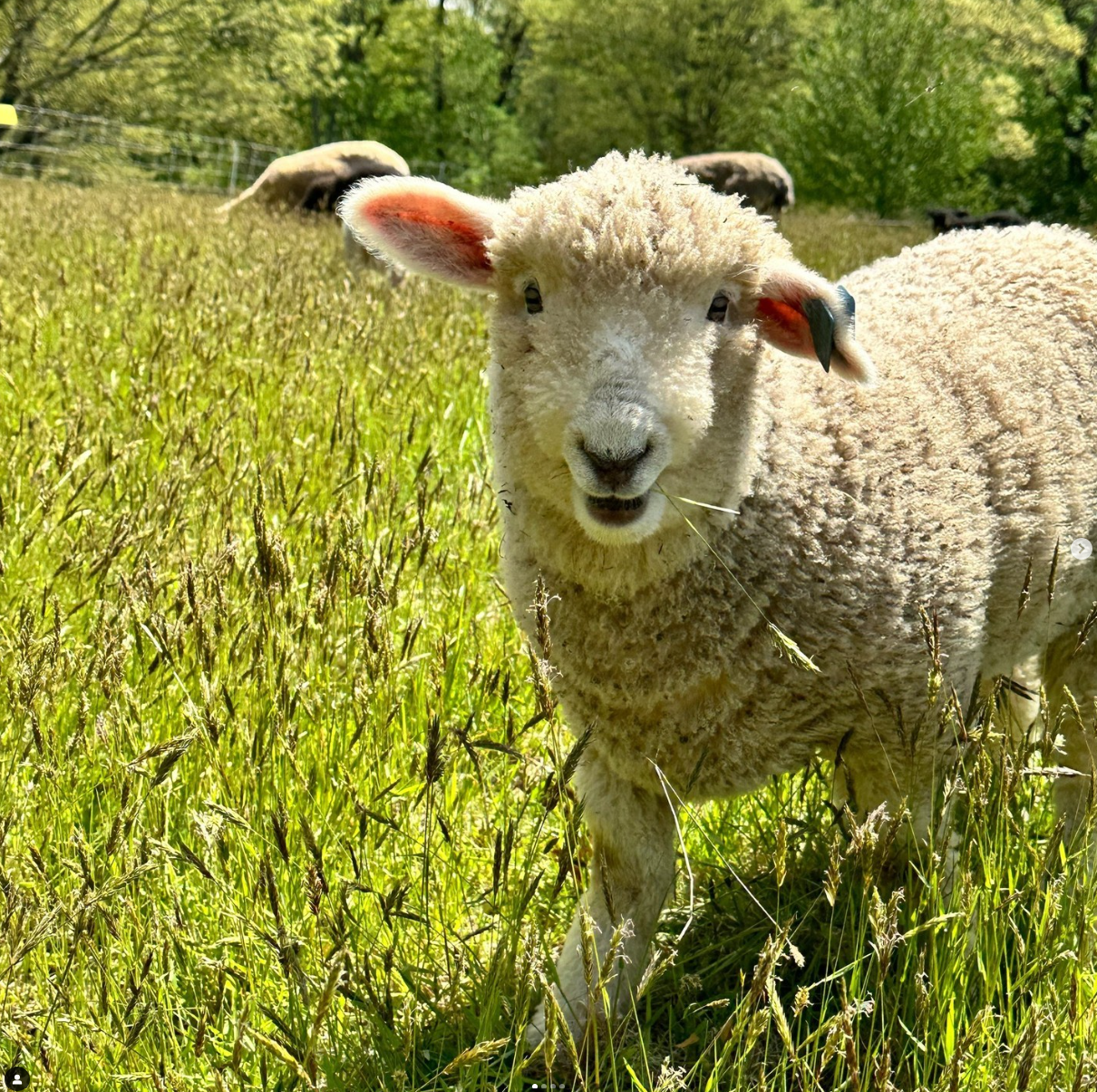
Drumlin Farm has welcomed MATLAMB, named in honor of MathWorks, among ten adorable new lambs this season!
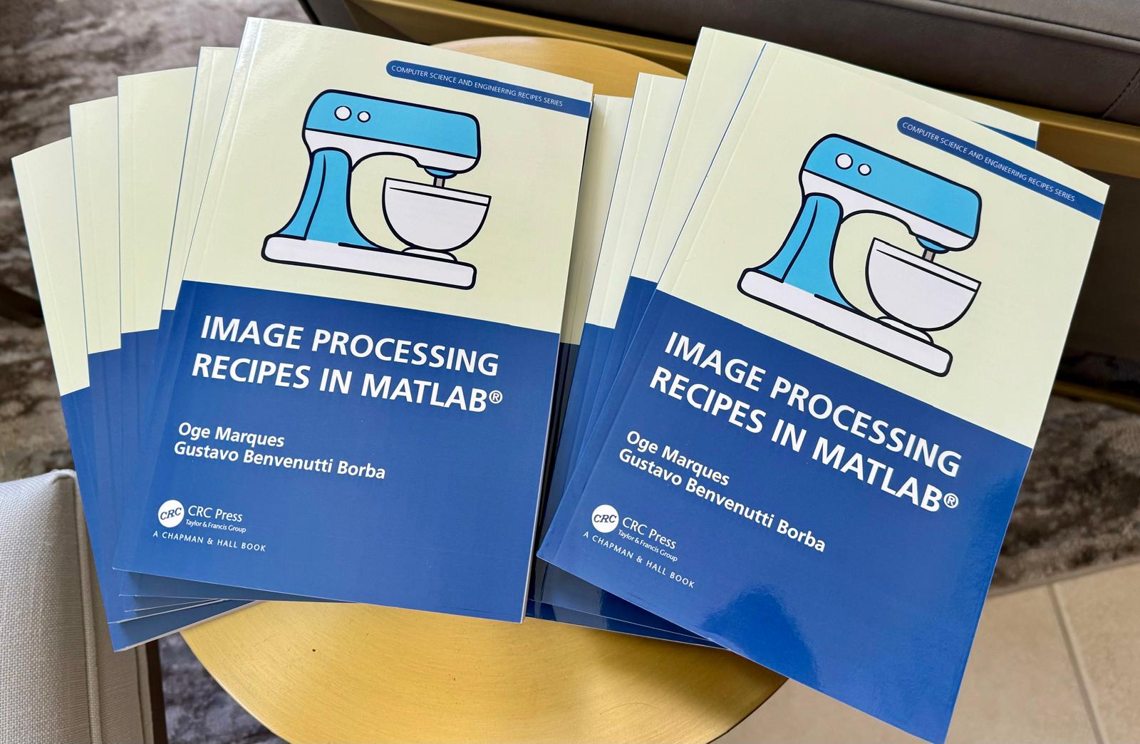
📚 New Book Announcement: "Image Processing Recipes in MATLAB" 📚
I am delighted to share the release of my latest book, "Image Processing Recipes in MATLAB," co-authored by my dear friend and colleague Gustavo Benvenutti Borba.
This 'cookbook' contains 30 practical recipes for image processing, ranging from foundational techniques to recently published algorithms. It serves as a concise and readable reference for quickly and efficiently deploying image processing pipelines in MATLAB.
Gustavo and I are immensely grateful to the MathWorks Book Program for their support. We also want to thank Randi Slack and her fantastic team at CRC Press for their patience, expertise, and professionalism throughout the process.
___________
A colleague said that you can search the Help Center using the phrase 'Introduced in' followed by a release version. Such as, 'Introduced in R2022a'. Doing this yeilds search results specific for that release.
Seems pretty handy so I thought I'd share.
Bringing the beauty of MathWorks Natick's tulips to life through code!
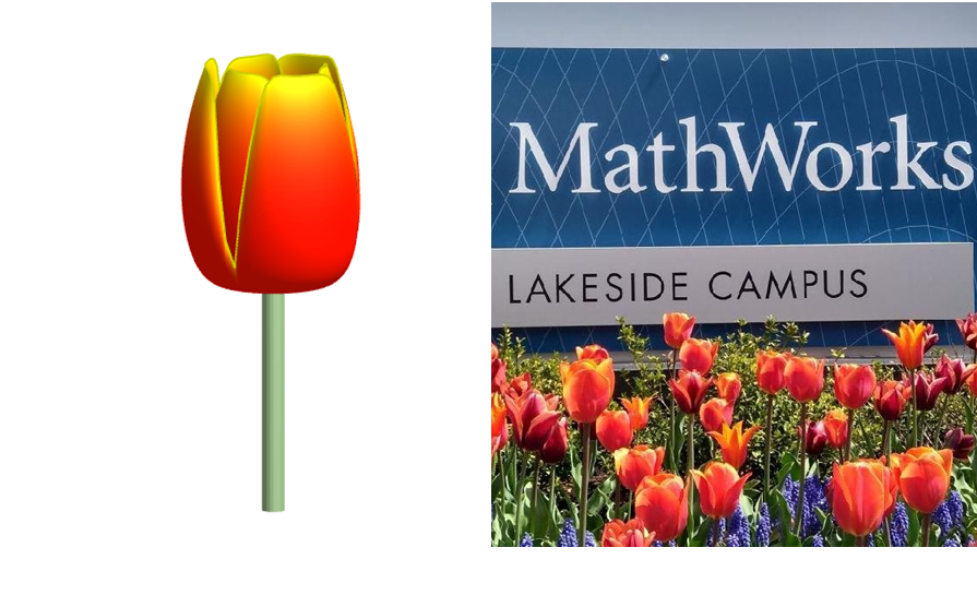
Remix challenge: create and share with us your new breeds of MATLAB tulips!
Hello MATLAB community,
I am doing some image processing with MATLAB and some issues with my coding. I just like to warn you that I am very new at coding and MATLAB so I apologise in advance for my low level and I would be very glad to have some help as I have hitted a wall, and can't find a solution to my problem.
Context: I have a video of beams, that move right to left over time. The base is fixed, only the beam moves. I converted the video to images, and my MATLAB program is going through the image file and treating every image in it. Here are two image examples:
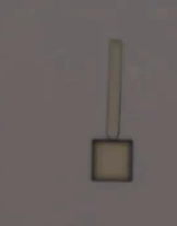 and
and 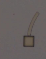
I want to measure the following things:
a. The coordinates between the 2 extremities of the beam (length of the beam, without its base), let's call them A and B.
b. The bending deformation E (L0-Lt/L0 *100), obtained by calculating the distance between A and B, called Lt.
c. the curvature of the beam (1/R), obtained by extracting the radius R of a circle fitting the curvature of the beam.
d. The angle between a vertical line passing through A, and the line AB.
What I have done so far:
My approach has been to transform my image into an rgbimage, then binaryImage, then have the complementary image, apply some modifications/corrections to the image, and then skeletonize it. And from then, I extract the coordinates of A and B, the distance between A&B (Lt), the radius of the beam R, and the angle between A&B (T).
My main issue is the skeletonisation. Because my beam is quite thick, it shortens up too much my beam, and in an inconcistent manner. So then my results are completly wrong. Here is an image of the different images and operation I have done and the result:
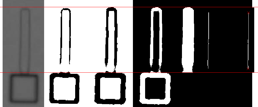
So as you can see, the length is shorter. I would like to have a skeleton that meets the edges of the beam to calculate the end points.
I have tried "bwskel(BW, 'MinBranchLength', 30)" and "bwmorph(BW, 'thin', inf)", and this: https://uk.mathworks.com/matlabcentral/fileexchange/11123-better-skeletonization. But the problem remains the same. I have tried regionpropos, but the major axis they return is too long, I have tried bwferet(), but the maxlength is in diagonal of the beam... I have running out of ideas.
Problem: So I guess my main problem is how can I get a skeletonisation that goes to the edges of the beam?
Here is my code:
for i = TrackingStart:TrackingEnd
FileRGB(:,:,i) = rgb2gray(imread(IMG)); % Convert to grayscale
croppedRGB = FileRGB(y3left:y3right, x3left:x3right, i);
binaryImage = imbinarize(croppedRGB, 'adaptive', 'ForegroundPolarity','dark','Sensitivity', 0.50);
out = nnz(~binaryImage);
while out <= 4300 % Change threshold if needed
for j = 1:50
sensitivity = 0.50 + j * 0.01;
binaryImage = imbinarize(croppedRGB, 'adaptive', 'ForegroundPolarity', 'dark', 'Sensitivity', sensitivity);
out = nnz(~binaryImage);
if out >= 4325
break; % Exit the loop if the condition is met
end
end
end
% Create a line Model
BW = imcomplement(binaryImage);
BW(y1left:y1right, x1left:x1right) = 1; % there is always sample at the junction area (between beam and base)
BW(y2left:y2right, x2left:x2right) = 0; % Always = 0 if no sample here
BW = bwmorph(BW, 'close', Inf);
BW = bwmorph(BW, 'bridge');
BW = bwareafilt(BW, 1);
s = regionprops(BW, 'FilledImage');
BW = s.FilledImage;
BW = bwskel(BW, 'MinBranchLength', 30);
endpoints = bwmorph(BW, 'endpoints');
[y_end, x_end] = find(endpoints == 1);
%Degree of bending deformation method
Lt = sqrt(power(x_end(1)-x_end(2),2)+power(y_end(1)-y_end(2),2));
if x_end(2) > x_end(1)
Lt = -Lt;
end
Lstore(i) = Lt;
%Curvature method
[row_dots_cir, col_dots_cir, val] = find(BW == 1);
[xc(i),yc(i),Rstore(i),a] = circfit(col_dots_cir,row_dots_cir);
%Angle method
slope_endpoints = (x_end(1) - x_end(2)) / (y_end(1) - y_end(2));
angle_radians = atan(slope_endpoints);
angle_degrees = rad2deg(angle_radians);
if x_end(2) > x_end(1)
angle_degrees = -angle_degrees;
end
Tstore(i) = angle_degrees;
i
end
I found this plot of words said by different characters on the US version of The Office sitcom. There's a sparkline for each character from pilot to finale episode.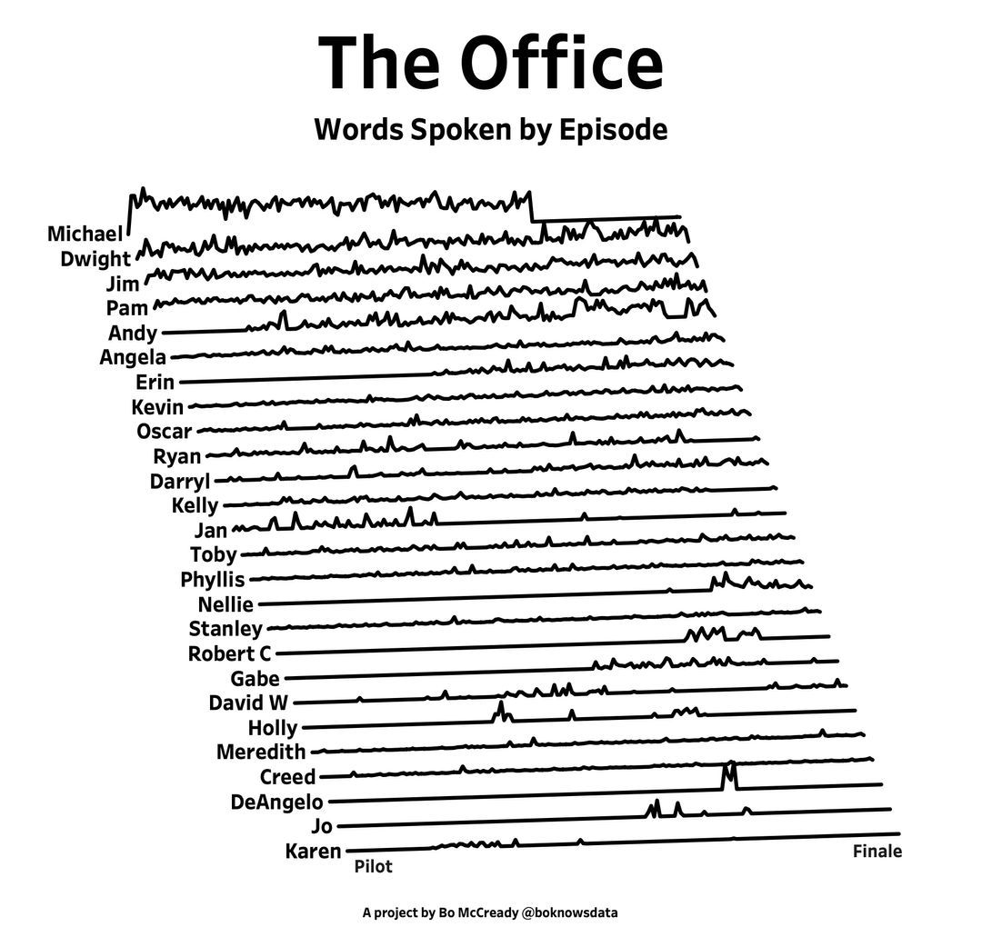
A high school student called for help with this physics problem:
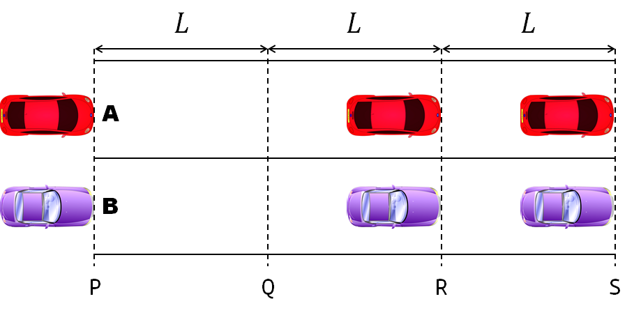
- Car A moves with constant velocity v.
- Car B starts to move when Car A passes through the point P.
- Car B undergoes...
- uniform acc. motion from P to Q.
- uniform velocity motion from Q to R.
- uniform acc. motion from R to S.
- Car A and B pass through the point R simultaneously.
- Car A and B arrive at the point S simultaneously.
Q1. When car A passes the point Q, which is moving faster?
Q2. Solve the time duration for car B to move from P to Q using L and v.
Q3. Magnitude of acc. of car B from P to Q, and from R to S: which is bigger?
Well, it can be solved with a series of tedious equations. But... how about this?
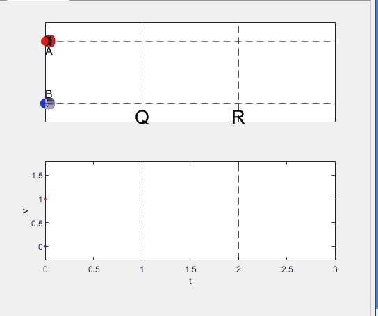
Code below:
%% get images and prepare stuffs
figure(WindowStyle="docked"),
ax1 = subplot(2,1,1);
hold on, box on
ax1.XTick = [];
ax1.YTick = [];
A = plot(0, 1, 'ro', MarkerSize=10, MarkerFaceColor='r');
B = plot(0, 0, 'bo', MarkerSize=10, MarkerFaceColor='b');
[carA, ~, alphaA] = imread('https://cdn.pixabay.com/photo/2013/07/12/11/58/car-145008_960_720.png');
[carB, ~, alphaB] = imread('https://cdn.pixabay.com/photo/2014/04/03/10/54/car-311712_960_720.png');
carA = imrotate(imresize(carA, 0.1), -90);
carB = imrotate(imresize(carB, 0.1), 180);
alphaA = imrotate(imresize(alphaA, 0.1), -90);
alphaB = imrotate(imresize(alphaB, 0.1), 180);
carA = imagesc(carA, AlphaData=alphaA, XData=[-0.1, 0.1], YData=[0.9, 1.1]);
carB = imagesc(carB, AlphaData=alphaB, XData=[-0.1, 0.1], YData=[-0.1, 0.1]);
txtA = text(0, 0.85, 'A', FontSize=12);
txtB = text(0, 0.17, 'B', FontSize=12);
yline(1, 'r--')
yline(0, 'b--')
xline(1, 'k--')
xline(2, 'k--')
text(1, -0.2, 'Q', FontSize=20, HorizontalAlignment='center')
text(2, -0.2, 'R', FontSize=20, HorizontalAlignment='center')
% legend('A', 'B') % this make the animation slow. why?
xlim([0, 3])
ylim([-.3, 1.3])
%% axes2: plots velocity graph
ax2 = subplot(2,1,2);
box on, hold on
xlabel('t'), ylabel('v')
vA = plot(0, 1, 'r.-');
vB = plot(0, 0, 'b.-');
xline(1, 'k--')
xline(2, 'k--')
xlim([0, 3])
ylim([-.3, 1.8])
p1 = patch([0, 0, 0, 0], [0, 1, 1, 0], [248, 209, 188]/255, ...
EdgeColor = 'none', ...
FaceAlpha = 0.3);
%% solution
v = 1; % car A moves with constant speed.
L = 1; % distances of P-Q, Q-R, R-S
% acc. of car B for three intervals
a(1) = 9*v^2/8/L;
a(2) = 0;
a(3) = -1;
t_BatQ = sqrt(2*L/a(1)); % time when car B arrives at Q
v_B2 = a(1) * t_BatQ; % speed of car B between Q-R
%% patches for velocity graph
p2 = patch([t_BatQ, t_BatQ, t_BatQ, t_BatQ], [1, 1, v_B2, v_B2], ...
[248, 209, 188]/255, ...
EdgeColor = 'none', ...
FaceAlpha = 0.3);
p3 = patch([2, 2, 2, 2], [1, v_B2, v_B2, 1], [194, 234, 179]/255, ...
EdgeColor = 'none', ...
FaceAlpha = 0.3);
%% animation
tt = linspace(0, 3, 2000);
for t = tt
A.XData = v * t;
vA.XData = [vA.XData, t];
vA.YData = [vA.YData, 1];
if t < t_BatQ
B.XData = 1/2 * a(1) * t^2;
vB.XData = [vB.XData, t];
vB.YData = [vB.YData, a(1) * t];
p1.XData = [0, t, t, 0];
p1.YData = [0, vB.YData(end), 1, 1];
elseif t >= t_BatQ && t < 2
B.XData = L + (t - t_BatQ) * v_B2;
vB.XData = [vB.XData, t];
vB.YData = [vB.YData, v_B2];
p2.XData = [t_BatQ, t, t, t_BatQ];
p2.YData = [1, 1, vB.YData(end), vB.YData(end)];
else
B.XData = 2*L + v_B2 * (t - 2) + 1/2 * a(3) * (t-2)^2;
vB.XData = [vB.XData, t];
vB.YData = [vB.YData, v_B2 + a(3) * (t - 2)];
p3.XData = [2, t, t, 2];
p3.YData = [1, 1, vB.YData(end), v_B2];
end
txtA.Position(1) = A.XData(end);
txtB.Position(1) = B.XData(end);
carA.XData = A.XData(end) + [-.1, .1];
carB.XData = B.XData(end) + [-.1, .1];
drawnow
end
I have question about using 'bnlssm' object when the problem involves time-varying coefs. Per this documentation https://www.mathworks.com/help/econ/bnlssm.html , bnlssm allows the transition matrix to be a nonlinear function of the past values of the state vector, while also being time-varying --, i.e. A_t(x_{t-1}). However the documentation contains an example of the parameter mapping function for a fixed coef. case only:
function [A,B,C,D,Mean0,Cov0,StateType] = paramMap(theta)
A = @(x)blkdiag([theta(1) theta(2); 0 1],[theta(3) theta(4); 0 1])*x;
B = [theta(5) 0; 0 0; 0 theta(6); 0 0];
C = @(x)log(exp(x(1)-theta(2)/(1-theta(1))) + ...
exp(x(3)-theta(4)/(1-theta(3))));
D = theta(7);
Mean0 = [theta(2)/(1-theta(1)); 1; theta(4)/(1-theta(3)); 1];
Cov0 = diag([theta(5)^2/(1-theta(1)^2) 0 theta(6)^2/(1-theta(3)^2) 0]);
StateType = [0; 1; 0; 1]; % Stationary state and constant 1 processes
end
Here, A and C are recognised as function handles and show the dimension of 1-by-1 when [A,B,C,D]=paramMap(theta) is run with a given theta. This does not prevent filter/smooth from returning the states estimates, as the function handles become m-by-m matices when the function handles are evaluated.
However, whenever I try replaceing A with a cell array, e.g.:
A=cell(T,1);
for t=1:T
A{t} = @(x)blkdiag([theta(1) theta(2); 0 1],[theta(3) theta(4); 0 1])*x;
end
bnlssm.fixcoeff throws an error that the dimensions of Mean0 are expected to be 1, per validation step in lines 700-707 of 'bnlssm.m':
if iscellA; At = A{1};
else; At = A; end
numStates0 = size(At,2);
if
isscalar(mean0)
mean0 = mean0(ones(numStates0,1),:);
elseif
~isempty(mean0)
mean0 = mean0(:);
validateattributes(mean0,{'numeric'},{'finite','real','numel',numStates0},callerName,'Mean0');
end
Q: Is it just overlook by MathWorks programmers and creating local verions of bnlssm/filter/smooth with that validation step removed is a viable pathway forward, or is it intentional because 'bnlssm' was in fact designed to handle only the time-invariant coef. case correctly?
From Alpha Vantage's website: API Documentation | Alpha Vantage
Try using the built-in Matlab function webread(URL)... for example:
% copy a URL from the examples on the site
URL = 'https://www.alphavantage.co/query?function=TIME_SERIES_DAILY&symbol=IBM&apikey=demo'
% or use the pattern to create one
tickers = [{'IBM'} {'SPY'} {'DJI'} {'QQQ'}]; i = 1;
URL = ...
['https://www.alphavantage.co/query?function=TIME_SERIES_DAILY_ADJUSTED&outputsize=full&symbol=', ...
+ tickers{i}, ...
+ '&apikey=***Put Your API Key here***'];
X = webread(URL);
You can access any of the data available on the site as per the Alpha Vantage documentation using these two lines of code but with different designations for the requested data as per the documentation.
It's fun!
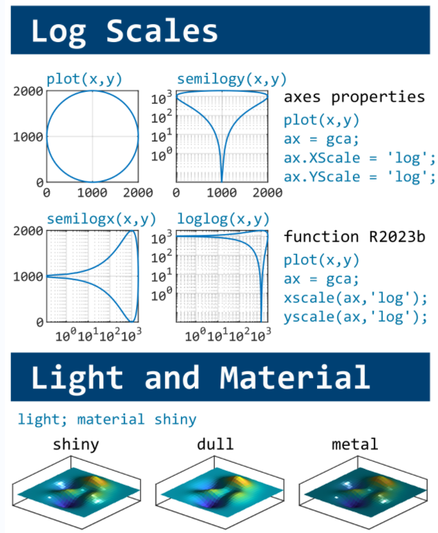
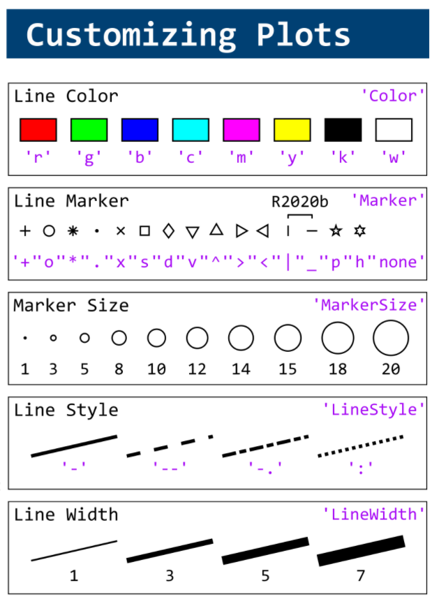
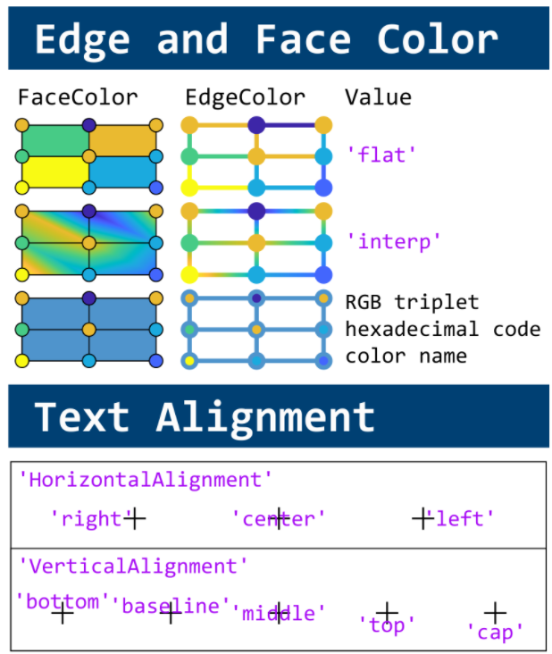
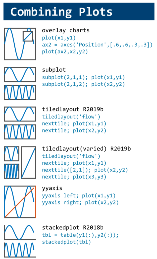
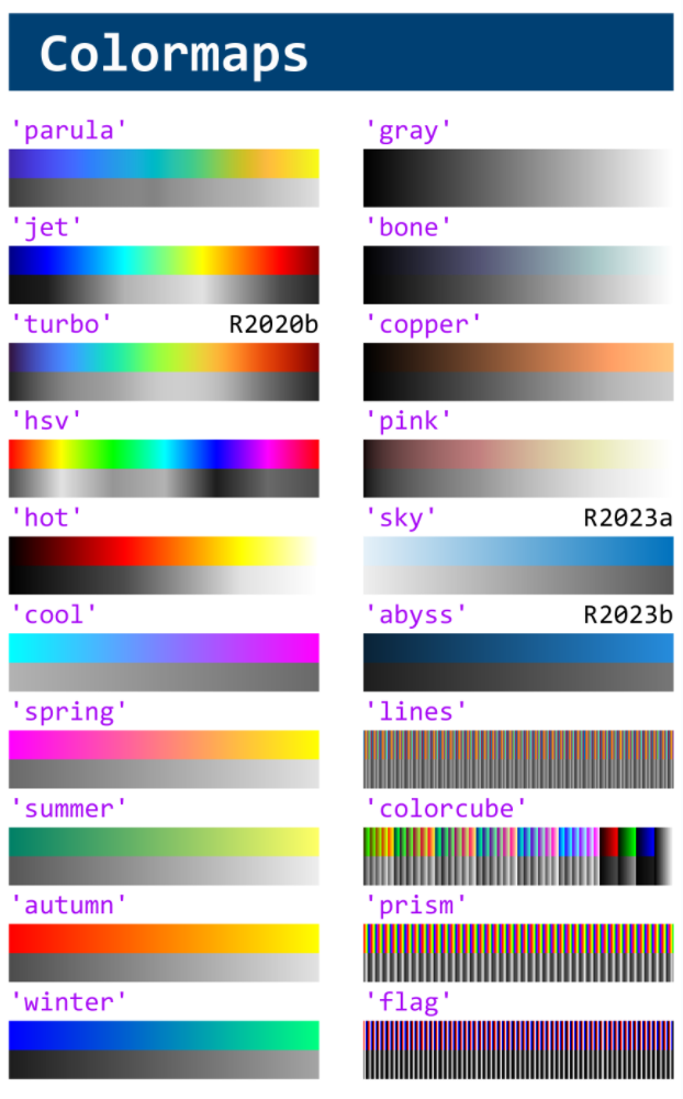
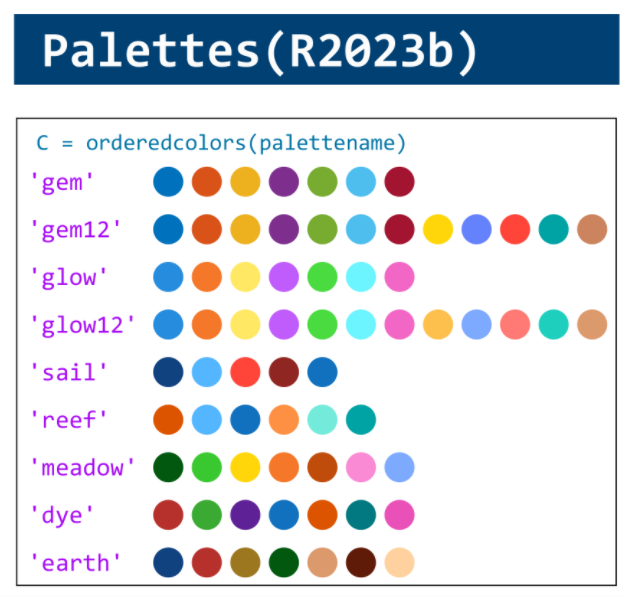
This cheat sheet is here:
reference:
- https://github.com/peijin94/matlabPlotCheatsheet
- https://github.com/mathworks/visualization-cheat-sheet
- https://www.mathworks.com/products/matlab/plot-gallery.html
- https://www.mathworks.com/help/matlab/release-notes.html
MATLAB used to have official visualization-cheat-sheet, but there have been quite a few new updates in MATLAB versions recently. Therefore, I made my own cheat sheet and marked the versions of each new thing that were released :
If structure is in the form of struct1.struct2(m,n).struct3. how to extract values present in struct3 using mex function