1922760350154212639070
メインコンテンツ
結果:
How can we use roughness in an effective context to identify large primes? I can quickly think of quite a few examples where we might do so. Again, remember I will be looking for primes with not just hundreds of decimal digits, or even only a few thousand digits. The eventual target is higher than that. Forget about targets for now though, as this is a journey, and what matters in this journey is what we may learn along the way.
I think the most obvious way to employ roughness is in a search for twin primes. Though not yet proven, the twin prime conjecture:
If it is true, it tells us there are infinitely many twin prime pairs. A twin prime pair is two integers with a separation of 2, such that both of them are prime. We can find quite a few of them at first, as we have {3,5}, {5,7}, {11,13}, etc. But there is only ONE pair of integers with a spacing of 1, such that both of them are prime. That is the pair {2,3}. And since primes are less and less common as we go further out, possibly there are only a finite number of twins with a spacing of exactly 2? Anyway, while I'm fairly sure the twin prime conjecture will one day be shown to be true, it can still be interesting to search for larger and larger twin prime pairs. The largest such known pair at the moment is
2996863034895*2^1290000 +/- 1
This is a pair with 388342 decimal digits. And while seriously large, it is still in range of large integers we can work with in MATLAB, though certainly not in double precision. In my own personal work on my own computer, I've done prime testing on integers (in MATLAB) with considerably more than 100,000 decimal digits.
But, again you may ask, just how does roughness help us here? In fact, this application of roughness is not new with me. You might want to read about tools like NewPGen {https://t5k.org/programs/NewPGen/} which sieves out numbers known to be composite, before any direct tests for primality are performed.
Before we even try to talk about numbers with thousands or hundreds of thousands of decimal digits, look at 6=2*3. You might observe
isprime([-1,1] + 6)
shows that both 5 and 7 are prime. This should not be a surprise, but think about what happens, about why it generated a twin prime pair. 6 is divisible by both 2 and 3, so neither 5 or 7 can possibly be divisible by either small prime as they are one more or one less than a multiple of both 2 and 3. We can try this again, pushing the limits just a bit.
isprime([-1,1] + 2*3*5)
That is again interesting. 30=2*3*5 is evenly divisible by 2, 3, and 5. The result is both 29 and 31 are prime, because adding 1 or subtracting 1 from a multiple of 2, 3, or 5 will always result in a number that is not divisible by any of those small primes. The next larger prime after 5 is 7, but it cannot be a factor of 29 or 31, since it is greater than both sqrt(29) and sqrt(31).
We have quite efficiently found another twin prime pair. Can we take this a step further? 210=2*3*5*7 is the smallest such highly composite number that is divisible by all primes up to 7. Can we use the same trick once more?
isprime([-1,1] + 2*3*5*7)
And here the trick fails, because 209=11*19 is not in fact prime. However, can we use the large twin prime trick we saw before? Consider numbers of the form [-1,1]+a*210, where a is itself some small integer?
a = 2;
isprime([-1,1] + a*2*3*5*7)
I did not need to look far, only out to a=2, because both 419 and 421 are prime. You might argue we have formed a twin prime "factory", of sorts. Next, I'll go out as far as the product of all primes not exceeding 60. This is a number with 22 decimal digits, already too large to represent as a double, or even as uint64.
prod(sym(primes(60)))
a = find(all(isprime([-1;1] + prod(sym(primes(60)))*(1:100)),1))
That easily identifies 3 such twin prime pairs, each of which has roughly 23 decimal digits, each of which have the form a*1922760350154212639070+/-1. The twin prime factory is still working well. Going further out to integers with 37 decimal digits, we can easily find two more such pairs that employ the product of all primes not exceeding 100.
prod(sym(primes(100)))
a = find(all(isprime([-1;1] + prod(sym(primes(100)))*(1:100)),1))
This is in fact an efficient way of identifying large twin prime pairs, because it chooses a massively composite number as the product of many distinct small primes. Adding or subtracting 1 from such a number will result always in a rough number, not divisible by any of the primes employed. With a little more CPU time expended, now working with numbers with over 1000 decimal digits, I will claim this next pair forms a twin prime pair, and is the smallest such pair we can generate in this way from the product of the primes not exceeding 2500.
isprime(7826*prod(sym(primes(2500))) + [-1 1])
ans =
logical
1
Unfortunately, 1000 decimal digits is at or near the limit of what the sym/isprime tool can do for us. It does beg the question, asking if there are alternatives to the sym/isprime tool, as an isProbablePrime test, usually based on Miller-Rabin is often employed. But this is gist for yet another set of posts.
Anyway, I've done a search for primes of the form
a*prod(sym(primes(10000))) +/- 1
having gone out as far as a = 600000, with no success as of yet. (My estimate is I will find a pair by the time I get near 5e6 for a.) Anyway, if others can find a better way to search for large twin primes in MATLAB, or if you know of a larger twin prime pair of this extended form, feel free to chime in.
What is a rough number? What can they be used for? Today I'll take you down a journey into the land of prime numbers (in MATLAB). But remember that a journey is not always about your destination, but about what you learn along the way. And so, while this will be all about primes, and specifically large primes, before we get there we need some background. That will start with rough numbers.
Rough numbers are what I would describe as wannabe primes. Almost primes, and even sometimes prime, but often not prime. They could've been prime, but may not quite make it to the top. (If you are thinking of Marlon Brando here, telling us he "could've been a contender", you are on the right track.)
Mathematically, we could call a number k-rough if it is evenly divisible by no prime smaller than k. (Some authors will use the term k-rough to denote a number where the smallest prime factor is GREATER than k. The difference here is a minor one, and inconsequential for my purposes.) And there are also smooth numbers, numerical antagonists to the rough ones, those numbers with only small prime factors. They are not relevant to the topic today, even though smooth numbers are terribly valuable tools in mathematics. Please forward my apologies to the smooth numbers.
Have you seen rough numbers in use before? Probably so, at least if you ever learned about the sieve of Eratosthenes for prime numbers, though probably the concept of roughness was never explicitly discussed at the time. The sieve is simple. Suppose you wanted a list of all primes less than 100? (Without using the primes function itself.)
% simple sieve of Eratosthenes
Nmax = 100;
N = true(1,Nmax); % A boolean vector which when done, will indicate primes
N(1) = false; % 1 is not a prime by definition
nextP = find(N,1,'first'); % the first prime is 2
while nextP <= sqrt(Nmax)
% flag multiples of nextP as not prime
N(nextP*nextP:nextP:end) = false;
% find the first element after nextP that remains true
nextP = nextP + find(N(nextP+1:end),1,'first');
end
primeList = find(N)
Indeed, that is the set of all 25 primes not exceeding 100. If you think about how the sieve worked, it first found 2 is prime. Then it discarded all integer multiples of 2. The first element after 2 that remains as true is 3. 3 is of course the second prime. At each pass through the loop, the true elements that remain correspond to numbers which are becoming more and more rough. By the time we have eliminated all multiples of 2, 3, 5, and finally 7, everything else that remains below 100 must be prime! The next prime on the list we would find is 11, but we have already removed all multiples of 11 that do not exceed 100, since 11^2=121. For example, 77 is 11*7, but we already removed it, because 77 is a multiple of 7.
Such a simple sieve to find primes is great for small primes. However is not remotely useful in terms of finding primes with many thousands or even millions of decimal digits. And that is where I want to go, eventually. So how might we use roughness in a useful way? You can think of roughness as a way to increase the relative density of primes. That is, all primes are rough numbers. In fact, they are maximally rough. But not all rough numbers are primes. We might think of roughness as a necessary, but not sufficient condition to be prime.
How many primes lie in the interval [1e6,2e6]?
numel(primes(2e6)) - numel(primes(1e6))
There are 70435 primes greater than 1e6, but less than 2e6. Given there are 1 million natural numbers in that set, roughly 7% of those numbers were prime. Next, how many 100-rough numbers lie in that same interval?
N = (1e6:2e6)';
roughInd = all(mod(N,primes(100)) > 0,2);
sum(roughInd)
That is, there are 120571 100-rough numbers in that interval, but all those 70435 primes form a subset of the 100-rough numbers. What does this tell us? Of the 1 million numbers in that interval, approximately 12% of them were 100-rough, but 58% of the rough set were prime.
The point being, if we can efficiently identify a number as being rough, then we can substantially increase the chance it is also prime. Roughness in this sense is a prime densifier. (Is that even a word? It is now.) If we can reduce the number of times we need to perform an explicit isprime test, that will gain greatly because a direct test for primality is often quite costly in CPU time, at least on really large numbers.
In my next post, I'll show some ways we can employ rough numbers to look for some large primes.
Do you boast about the energy savings you racking up by using dark mode while stashing your energy bill savings away for an exotic vacation🌴🥥? Well, hold onto your sun hats and flipflops!
A recent study presented at the 1st Internaltional Workshop on Low Carbon Computing suggests that you may be burning more ⚡energy⚡ with your slick dark displays 💻[1].
In a 2x2 factorial design, ten participants viewed a webpage in dark and light modes in both dim and lit settings using an LCD monitor with 16 brightness levels.
- 80% of participants increased the monitor's brightness in dark mode [2]
- This occurred in both lit and dim rooms
- Dark mode did not reduce power draw but increasing monitor brightness did.
The color pixels in an LCD monitor still draw voltage when the screen is black, which is why the monitor looks gray when displaying a pure black background in a dark room. OLED monitors, on the other hand, are capable of turning off pixels that represent pure black and therefore have the potential to save energy with dark mode. A 2021 Purdue study estimates a 3%-9% energy savings with dark mode on OLED monitors using auto-brightness [3]. However, outside of gaming, OLED monitors have a very small market share and still account for less than 25% within the gaming world.
Any MATLAB users out there with OLED monitors? How are you going to spend your mad cash savings when you start using MATLAB's upcoming dark theme?
- BBC study: https://www.sicsa.ac.uk/wp-content/uploads/2024/11/LOCO2024_paper_12.pdf
- BBC blog article https://www.bbc.co.uk/rd/articles/2025-01-sustainability-web-energy-consumption
- 2021 Purdue https://dl.acm.org/doi/abs/10.1145/3458864.3467682
I've been trying this problem a lot of time and i don't understand why my solution doesnt't work.
In 4 tests i get the error Assertion failed but when i run the code myself i get the diag and antidiag correctly.
function [diag_elements, antidg_elements] = your_fcn_name(x)
[m, n] = size(x);
% Inicializar los vectores de la diagonal y la anti-diagonal
diag_elements = zeros(1, min(m, n));
antidg_elements = zeros(1, min(m, n));
% Extraer los elementos de la diagonal
for i = 1:min(m, n)
diag_elements(i) = x(i, i);
end
% Extraer los elementos de la anti-diagonal
for i = 1:min(m, n)
antidg_elements(i) = x(m-i+1, i);
end
end
On 27th February María Elena Gavilán Alfonso and I will be giving an online seminar that has been a while in the making. We'll be covering MATLAB with Jupyter, Visual Studio Code, Python, Git and GitHub, how to make your MATLAB projects available to the world (no installation required!) and much much more.
Sign up (it's free!) at MATLAB Without Borders: Connecting your Projects with Python and other Open-Source Tools - MATLAB & Simulink

I am looking for a Simulink tutor to help me with Reinforcement Learning Agent integration. If you work for MathWorks, I am willing to pay $30/hr. I am working on a passion project, ready to start ASAP. DM me if you're interested.
Bitte um Hilfe beim Kauf
Since May 2023, MathWorks officially introduced the new Community API(MATLAB Central Interface for MATLAB), which supports both MATLAB and Node.js languages, allowing users to programmatically access data from MATLAB Answers, File Exchange, Blogs, Cody, Highlights, and Contests.
I’m curious about what interesting things people generally do with this API. Could you share some of your successful or interesting experiences? For example, retrieving popular Q&A topics within a certain time frame through the API and displaying them in a chart.
If you have any specific examples or ideas in mind, feel free to share!
On my computers, this bit of code produces an error whose cause I have pinpointed,
load tstcase
ycp=lsqlin(I, y, Aineq, bineq);
Error using parseOptions
Too many output arguments.
Error in lsqlin (line 170)
[options, optimgetFlag] = parseOptions(options, 'lsqlin', defaultopt);
^^^^^^^^^^^^^^^^^^^^^^^^^^^^^^^^^^^^^^^^^^^
The reason for the error is seemingly because, in recent Matlab, lsqlin now depends on a utility function parseOptions, which is shadowed by one of my personal functions sharing the same name:
C:\Users\MWJ12\Documents\mwjtree\misc\parseOptions.m
C:\Program Files\MATLAB\R2024b\toolbox\shared\optimlib\parseOptions.m % Shadowed
The MathWorks-supplied version of parseOptions is undocumented, and so is seemingly not meant for use outside of MathWorks. Shouldn't it be standard MathWorks practice to put these utilities in a private\ folder where they cannot conflict with user-supplied functions of the same name?
It is going to be an enormous headache for me to now go and rename all calls to my version of parseOptions. It is a function I have been using for a long time and permeates my code.
General observations on practical implementation issues regarding add-on versioning
I am making updates to one of my File Exchange add-ons, and the updates will require an updated version of another add-on. The state of versioning for add-ons seems to be a bit of a mess.
First, there are several sources of truth for an add-on’s version:
- The GitHub release version, which gets mirrored to the File Exchange version
- The ToolboxVersion property of toolboxOptions (for an add-on packaged as a toolbox)
- The version in the Contents.m file (if there is one)
Then, there is the question of how to check the version of an installed add-on. You can call matlab.addon.installedAddons, which returns a table. Then you need to inspect the table to see if a particular add-on is present, if it is enabled, and get the version number.
If you can get the version number this way, then you need some code to compare two semantic version numbers (of the form “3.1.4”). I’m not aware of a documented MATLAB function for this. The verLessThan function takes a toolbox name and a version; it doesn’t help you with comparing two versions.
If add-on files were downloaded directly and added to the MATLAB search path manually, instead of using the .mtlbx installer file, the add-on won’t be listed in the table returned by matlab.addon.installedAddon. You’d have to call ver to get the version number from the Contents.m file (if there is one).
Frankly, I don’t want to write any of this code. It would take too long, be challenging to test, and likely be fragile.
Instead, I think I will write some sort of “capabilities” utility function for the add-on. This function will be used to query the presence of needed capabilities. There will still be a slight coding hassle—the client add-on will need to call the capabilities utility function in a try-catch, because earlier versions of the add-on will not have that utility function.
I also posted this over at Harmonic Notes
Simulink has been an essential tool for modeling and simulating dynamic systems in MATLAB. With the continuous advancements in AI, automation, and real-time simulation, I’m curious about what the future holds for Simulink.
What improvements or new features do you think Simulink will have in the coming years? Will AI-driven modeling, cloud-based simulation, or improved hardware integration shape the next generation of Simulink?
MATLAB FEX(MATLAB File Exchange) should support Markdown syntax for writing. In recent years, many open-source community documentation platforms, such as GitHub, have generally supported Markdown. MATLAB is also gradually improving its support for Markdown syntax. However, when directly uploading files to the MATLAB FEX community and preparing to write an overview, the outdated document format buttons are still present. Even when directly uploading a Markdown document, it cannot be rendered. We hope the community can support Markdown syntax!
BTW,I know that open-source Markdown writing on GitHub and linking to MATLAB FEX is feasible, but this is a workaround. It would be even better if direct native support were available.
You've probably heard about the DeepSeek AI models by now. Did you know you can run them on your own machine (assuming its powerful enough) and interact with them on MATLAB?
In my latest blog post, I install and run one of the smaller models and start playing with it using MATLAB.
Larger models wouldn't be any different to use assuming you have a big enough machine...and for the largest models you'll need a HUGE machine!
Even tiny models, like the 1.5 billion parameter one I demonstrate in the blog post, can be used to demonstrate and teach things about LLM-based technologies.
Have a play. Let me know what you think.
My following code works running Matlab 2024b for all test cases. However, 3 of 7 tests fail (#1, #4, & #5) the QWERTY Shift Encoder problem. Any ideas what I am missing?
Thanks in advance.
keyboardMap1 = {'qwertyuiop[;'; 'asdfghjkl;'; 'zxcvbnm,'};
keyboardMap2 = {'QWERTYUIOP{'; 'ASDFGHJKL:'; 'ZXCVBNM<'};
if length(s) == 0
se = s;
end
for i = 1:length(s)
if double(s(i)) >= 65 && s(i) <= 90
row = 1;
col = 1;
while ~strcmp(s(i), keyboardMap2{row}(col))
if col < length(keyboardMap2{row})
col = col + 1;
else
row = row + 1;
col = 1;
end
end
se(i) = keyboardMap2{row}(col + 1);
elseif double(s(i)) >= 97 && s(i) <= 122
row = 1;
col = 1;
while ~strcmp(s(i), keyboardMap1{row}(col))
if col < length(keyboardMap1{row})
col = col + 1;
else
row = row + 1;
col = 1;
end
end
se(i) = keyboardMap1{row}(col + 1);
else
se(i) = s(i);
end
% if ~(s(i) = 65 && s(i) <= 90) && ~(s(i) >= 97 && s(i) <= 122)
% se(i) = s(i);
% end
end
Currently, according to the official documentation, "DisplayName" only supports character vectors or single scalar string as input. For example, when plotting three variables simultaneously, if I use a single scalar string as input, the legend labels will all be the same. To have different labels, I need to specify them separately using the legend function with label1, label2, label3.
Here's an example illustrating the issue:
x = (1:10)';
y1 = x;
y2 = x.^2;
y3 = x.^3;
% Plotting with a string scalar for DisplayName
figure;
plot(x, [y1,y2,y3], DisplayName="y = x");
legend;
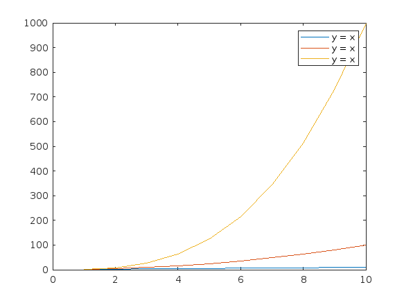
% To have different labels, I need to use the legend function separately
figure;
plot(x, [y1,y2,y3], DisplayName=["y = x","y = x^2","y=x^3"]);
% legend("y = x","y = x^2","y=x^3");
Too small
22%
Just right
38%
Too large
40%
2648 票
In one of my MATLAB projects, I want to add a button to an existing axes toolbar. The function for doing this is axtoolbarbtn:
axtoolbarbtn(tb,style,Name=Value)
However, I have found that the existing interfaces and behavior make it quite awkward to accomplish this task.
Here are my observations.
Adding a Button to the Default Axes Toolbar Is Unsupported
plot(1:10)
ax = gca;
tb = ax.Toolbar
Calling axtoolbarbtn on ax results in an error:
>> axtoolbarbtn(tb,"state")
Error using axtoolbarbtn (line 77)
Modifying the default axes toolbar is not supported.
Default Axes Toolbar Can't Be Distinguished from an Empty Toolbar
The Children property of the default axes toolbar is empty. Thus, it appears programmatically to have no buttons, just like an empty toolbar created by axtoolbar.
cla
plot(1:10)
ax = gca;
tb = ax.Toolbar;
tb.Children
ans = 0x0 empty GraphicsPlaceholder array.
tb2 = axtoolbar(ax);
tb2.Children
ans = 0x0 empty GraphicsPlaceholder array.
A Workaround
An empty axes toolbar seems to have no use except to initalize a toolbar before immediately adding buttons to it. Therefore, it seems reasonable to assume that an axes toolbar that appears to be empty is really the default toolbar. While we can't add buttons to the default axes toolbar, we can create a new toolbar that has all the same buttons as the default one, using axtoolbar("default"). And then we can add buttons to the new toolbar.
That observation leads to this workaround:
tb = ax.Toolbar;
if isempty(tb.Children)
% Assume tb is the default axes toolbar. Recreate
% it with the default buttons so that we can add a new
% button.
tb = axtoolbar(ax,"default");
end
btn = axtoolbarbtn(tb);
% Then set up the button as desired (icon, callback,
% etc.) by setting its properties.
As workarounds go, it's not horrible. It just seems a shame to have to delete and then recreate a toolbar just to be able to add a button to it.
The worst part about the workaround is that it is so not obvious. It took me a long time of experimentation to figure it out, including briefly giving it up as seemingly impossible.
The documentation for axtoolbarbtn avoids the issue. The most obvious example to write for axtoolbarbtn would be the first thing every user of it will try: add a toolbar button to the toolbar that gets created automatically in every call to plot. The doc page doesn't include that example, of course, because it wouldn't work.
My Request
I like the axes toolbar concept and the axes interactivity that it promotes, and I think the programming interface design is mostly effective. My request to MathWorks is to modify this interface to smooth out the behavior discontinuity of the default axes toolbar, with an eye towards satisfying (and documenting) the general use case that I've described here.
One possible function design solution is to make the default axes toolbar look and behave like the toolbar created by axtoolbar("default"), so that it has Children and so it is modifiable.
I am curious as to how my goal can be accomplished in Matlab.
The present APP called "Matching Network Designer" works quite well, but it is limited to a single section of a "PI", a "TEE", or an "L" topology circuit.
This limits the bandwidth capability of the APP when the intended use is to create an amplifier design intended for wider bandwidth projects.
I am requesting that a "Broadband Matching Network Designer" APP be developed by you, the MathWorks support team.
One suggestion from me is to be able to cascade a second section (or "pole") to the first.
Then the resulting topology would be capable of achieving that wider bandwidth of the microwave amplifier project where it would be later used with the transistor output and input matching networks.
Instead of limiting the APP to a single frequency, the entire s parameter file would be used as an input.
The APP would convert the polar s parameters to rectangular scaler complex impedances that you already use.
At that point, having started out with the first initial center frequency, the other frequencies both greater than and less than the center would come into use by an optimization of the circuit elements.
I'm hoping that you will be able to take on this project.
I can include an attachment of such a Matching Network Designer APP that you presently have if you like.
That network is centered at 10 GHz.
Kimberly Renee Alvarez.
310-367-5768
私の場合、前の会社が音楽認識アプリの会社で、アルゴリズム開発でFFTが使われていたことがきっかけでした。でも、MATLABのすごさが分かったのは、機械学習のオンライン講座で、Andrew Ngが、線型代数を使うと、数式と非常に近い構文のコードで問題が処理できることを学んだ時でした。
また、以下のリストから Web サイトを選択することもできます。
南北アメリカ
- América Latina (Español)
- Canada (English)
- United States (English)
ヨーロッパ
- Belgium (English)
- Denmark (English)
- Deutschland (Deutsch)
- España (Español)
- Finland (English)
- France (Français)
- Ireland (English)
- Italia (Italiano)
- Luxembourg (English)
- Netherlands (English)
- Norway (English)
- Österreich (Deutsch)
- Portugal (English)
- Sweden (English)
- Switzerland
- United Kingdom(English)
アジア太平洋地域
- Australia (English)
- India (English)
- New Zealand (English)
- 中国
- 日本Japanese (日本語)
- 한국Korean (한국어)