メインコンテンツ
結果:
Calling all students! New to MATLAB or need helpful resources? Check out our MATLAB GitHub for Students repository! Find MATLAB examples, videos, cheat sheets, and more!

Visit the repository here: MATLAB GitHub for Students
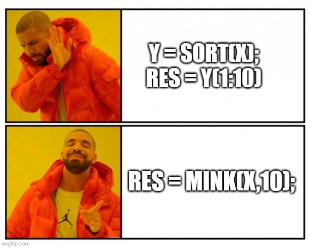
Imagine x is a large vector and you want the smallest 10 elements. How might you do it?
The way we've solved ODEs in MATLAB has been relatively unchanged at the user-level for decades. Indeed, I consider ode45 to be as iconic as backslash! There have been a few new solvers in recent years -- ode78 and ode89 for example -- and various things have gotten much faster but if you learned how to solve ODEs in MATLAB in 1997 then your knowledge is still applicable today.
In R2023b, there's a completely new framework for solving ODEs and I love it! You might argue that I'm contractually obliged to love it since I'm a MathWorker but I can assure you this is the real thing!
I wrote it up in a tutorial style on The MATLAB Blog https://blogs.mathworks.com/matlab/2023/10/03/the-new-solution-framework-for-ordinary-differential-equations-odes-in-matlab-r2023b/
The new interface makes a lot of things a much easier to do. Its also setting us up for a future where we'll be able to do some very cool algorithmic stuff behind the scenes.
Let me know what you think of the new functionality and what you think MathWorks should be doing next in the area of ODEs.
The new solution framework for Ordinary Differential Equations (ODEs) in MATLAB R2023b
Along with linear algebra, one of the iconic features of MATLAB in my mind is how it handles ordinary differential equations (ODEs). ODEs have been part of MATLAB almost since the very beginning.One of the features of how MATLAB traditionally allows users to solve ODEs is that it provides a suite of functions. For many years, there were 7
4 months ago, the new API was published to access content on the MATLAB Central community. I shared my MATLAB code to access the API at that time, but the team just released the official SDK.
MATLAB toolbox on File Exchange: https://www.mathworks.com/matlabcentral/fileexchange/135567-matlab-central-interface-for-matlab
MATLAB Central Interface for MATLAB
Toolbox to access MATLAB Central APIs from MATLAB
Houman and Rameez will talk about how you can model wireless networks (5G, WLAN, Bluetooth, 802.11ax WLAN mesh, etc.) in MATLAB in the upcoming livestream. They will start with the basics such as nodes, links, topology and metrics. Then they will introduce a new free add-on library that lets you model such networks, and show you how to use it.
- Date: Thu, Oct 5, 2023
- Time: 11 am EDT (or your local time)
Bookmark this link:

To solve the puzzle, first unscramble each of the words on the left. Then rearrange the letters in the yellow shaded boxes to complete the sentence on the right.
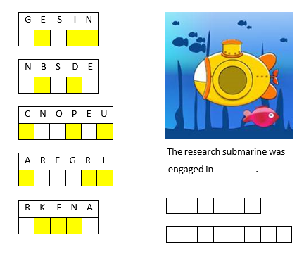
If you enjoyed this puzzle let me know with a like or in the comments below and I'll post more of them. Please don't post your answer, or any hints, and spoil it for those who come across this puzzle after you!! If you want to check your answer, you can messge me your guess through the link on my profile card (click on my name, Rena Berman, above and then on the envelope icon in the top right corner of the profile card that appears).
Congratulations, @Adam Danz for winning the Editor's Pick badge awarded for MATLAB Answers, in recognition of your awesome solution in overlapping images in grid layout.
Thank you for going to great lengths to help a user in this thread by suggesting alternative approach to representing stack of playing cards in MATLAB, highlighting very interesting features like hggroup.
This badge recognizes awesome answers people contribute and yours was picked for providing a very detailed and helpful answer.
Thank you so much for setting a high standard for MATLAB Answers and for your ongoing contribution to the community.
MATLAB Central Team

You had a meteoric rise to in our community since you started answering questions in June 2020.
You provided 3218 answers and 926 votes. You are ranked #23 in the community. Thank you for your contribution to the community and please keep up the good track record!
MATLAB Central Team
MATLAB Onramp is a free online tutorial and it has been very popular with new MATLAB users to learn how to use it, and MathWorks have been adding more and more modules. The lastest one just dropped https://matlabacademy.mathworks.com/details/power-systems-simulation-onramp/orps
It shows you the basics of power system simulation by modeling a simple microgrid. You will learn how to simulate and measure three-phase circuits, and how to evaluate algorithms like droop control and maximum power point tracking.
cities
15%
beaches, islands, or cruises
22%
rivers, lakes, or mountains
33%
National Parks or historical sites
14%
wherever my family lives
12%
somewhere else
5%
13709 票
I am trying to make a simulink model to use a MPC to reduce power consumption of HVAC system in an electric vehicle during cool down from ambient temperature to a set point temperature. Any help regarding this would be appreciated
Hi Everyone,
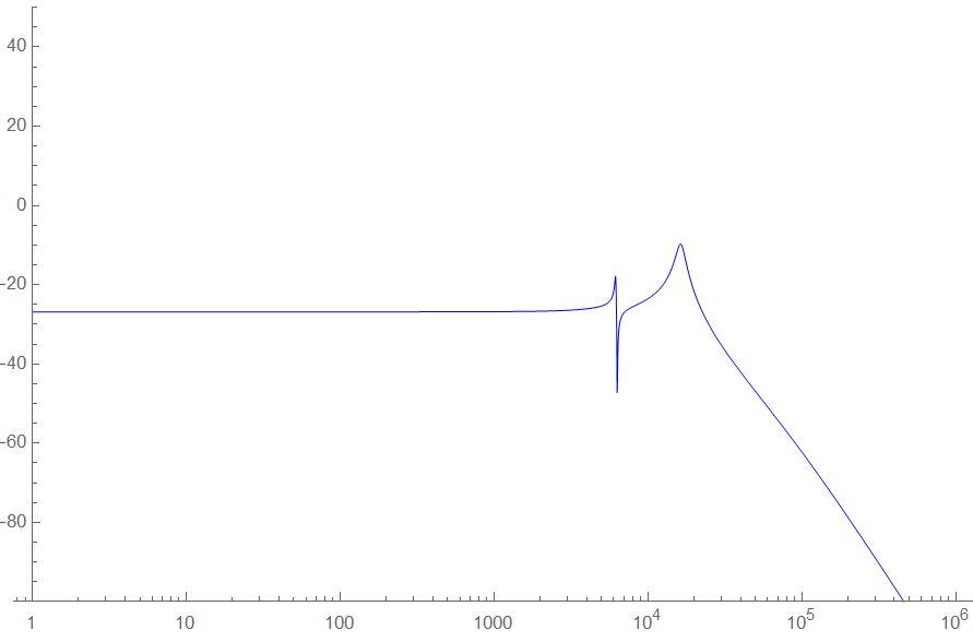
I have a high-order filter and I need to determinate its R,L,C values. In the simulation, the filter is unstable for some values. But I want to find values for stability of the filter. For second order system has some formulation between Q and phase margin so that it can be obtain the stability ciriteria to choose components.
My transfer function denominator is 5th order polynomial, and it is not possible to find roots in terms of R,L,C, Lm. I need to factor it like one 1th and two second order as shown in below.
D(s) = (1+s/wp) (1+s/wo1Q1 + (s/wo1)²) (1+s/wo2Q2 + (s/wo2)²)
Is there any methods to reduce order of transfer function?(Maybe, it can be possible for only in certain frequency range, can be renounced high-frequency )

Hello, an intern working at MathWorks is finishing up his program soon and he would like to interview some MATLAB users. He is looking for people who can give their perspective on the question:
"What makes MATLAB and Simulink special in comparison to other languages?"
Ultimately he plans to condense the answers into 15-second videos or sound bites.
If people are willing to participate but want more time to talk about their experience with MATLAB, he doesn't have time left for in-depth interviews but he can find someone else to take over the project.
Please send me an email via my profle if you are interested.
Yes, in my company that I own
35%
Yes, for someone else (or Univ.)
21%
Only for free, for charities
13%
Only in my charitable foundation
5%
No, I'd just play, travel, & relax
25%
15668 票
Kindly help me correct this code to function properly. I am just learning MATLAB. i cannot get the output in abc frame. This is the code:
%----------- Define input and state parameters-----------------------------
clc
v_dc = 350; % DC input voltage in V
m = 0.841; % modulation index
C = 4000e-6; % DC buss capacitance in uf
L_1 = 2.5e-3; % Inverter side inductance in mH
L_2 = 2.5e-3; % Load side inductance in mH
L = 0; % load inductance
C_f = 10e-6; % filter capacitance in uf
R_f = 0.7; % damping resistance in ohms
R_L = 20; % load resistance in ohms
f_s = 10e3; % switching frequency
f = 60; % System frequency
R_s = 0.01; % Capacitance of the DC circuit
I_d = 8.594; % steady state current
w = 2*pi*f; % System angular Frequency
% Define initial steady state values
v_c = 349.4; i_d = 8.594; i_q = -0.213; v_df = 285; v_qf = -120; i_Ld = 8.594; i_Lq = 0.85;
%------------------S V P W M Generator-------------------------------------
% Define reference vector Uref
U_mag = m*v_dc/2; % Magnitude of Uref
% Define switching vectors
U1 = [v_dc/2;0]; % Vector Q1
U2 = [v_dc/4;sqrt(3)*v_dc/4]; % Vector Q2
U3 = [-v_dc/4;sqrt(3)*v_dc/4]; % Vector Q3
U4 = [-v_dc/2;0]; % Vector Q4
U5 = [-v_dc/4;-sqrt(3)*v_dc/4]; % Vector Q5
U6 = [v_dc/4;-sqrt(3)*v_dc/4]; % Vector Q6
% Define sector angles
theta1 = pi/6;
theta2 = pi/2;
theta3 = 5*pi/6;
theta4 = 7*pi/6;
theta5 = 3*pi/2;
theta6 = 11*pi/6;
% Define duty cycles for each switch using a for loop
for t=0:1/f_s:1/f % Time variable from 0 to one cycle of system frequency with steps of switching frequency
U_phase = w*t; % Phase of Uref (t is time variable)
U_alpha = U_mag*cos(U_phase); % Alpha component of Uref
U_beta = U_mag*sin(U_phase); % Beta component of Uref
if (0 <= U_phase) && (U_phase < theta1) % Sector 1
T1 = (sqrt(3)*U_beta + U_alpha)/(2*v_dc);
T2 = (-sqrt(3)*U_beta + U_alpha)/(2*v_dc);
T0 = 1 - T1 - T2;
d_a(round(t)+1) = T1 + T0/2;
d_b(round(t)+1) = T2 + T0/2;
d_c(round(t)+1) = T0/2;
elseif (theta1 <= U_phase) && (U_phase < theta2) % Sector 2
T3 = (sqrt(3)*U_beta - U_alpha)/(2*v_dc);
T2 = (sqrt(3)*U_beta + U_alpha)/(2*v_dc);
T0 = 1 - T3 - T2;
d_a(round(t)+1) = T0/2;
d_b(round(t)+1) = T2 + T0/2;
d_c(round(t)+1) = T3 + T0/2;
elseif (theta2 <= U_phase) && (U_phase < theta3) % Sector 3
T3 = (sqrt(3)*U_beta - U_alpha)/(2*v_dc);
T4 = (-sqrt(3)*U_beta - U_alpha)/(2*v_dc);
T0 = 1 - T3 - T4;
d_a(round(t)+1) = T0/2;
d_b(round(t)+1) = T0/2;
d_c(round(t)+1) = T3 + T0/2;
elseif (theta3 <= U_phase) && (U_phase < theta4) % Sector 4
T5 = (-sqrt(3)*U_beta + U_alpha)/(2*v_dc);
T4 = (-sqrt(3)*U_beta - U_alpha)/(2*v_dc);
T0 = 1 - T5 - T4;
d_a(round(t)+1) = T5 + T0/2;
d_b(round(t)+1) = T0/2;
d_c(round(t)+1) = T4 + T0/2;
elseif (theta4 <= U_phase) && (U_phase < theta5) % Sector 5
T5 = (-sqrt(3)*U_beta + U_alpha)/(2*v_dc);
T6 = (sqrt(3)*U_beta + U_alpha)/(2*v_dc);
T0 = 1 - T5 - T6;
d_a(round(t)+1) = T5 + T0/2;
d_b(round(t)+1) = T6 + T0/2;
d_c(round(t)+1) = T0/2;
elseif (theta5 <= U_phase) && (U_phase < theta6) % Sector 6
T1 = (sqrt(3)*U_beta + U_alpha)/(2*v_dc);
T6 = (sqrt(3)*U_beta - U_alpha)/(2*v_dc);
T0 = 1 - T1 - T6;
d_a(round(t)+1) = T1 + T0/2;
d_b(round(t)+1) = T0/2;
d_c(round(t)+1) = T6 + T0/2;
end
end
%-------------------------Define system matrices---------------------------
% Create Three-phase SVPWM VSI Inverter
% System matrix Nx-by-Nx matrix
A = [-1/(C*R_s),-sqrt(3)*m/(2*C),0,0,0,0,0;
sqrt(3)*m/(3*L_1),-R_f/(3*L_1),w,-1/(2*L_1),-sqrt(3)/(6*L_1),-R_f/(3*L_1),0;
0,-w,-R_f/(3*L_1),-sqrt(3)/(6*L_1),-1/(2*L_1),0,R_f/(3*L_1);
0,1/(2*C_f),-sqrt(3)/(6*C_f),0,w,-1/(2*C_f),sqrt(3)/(6*C_f);
0,sqrt(3)/(6*C_f),1/(2*C_f),-w,0,-sqrt(3)/(6*C_f),-1/(2*C_f);
0,R_f/(3*(L_2+L)),0,1/(2*(L_2+L)),sqrt(3)/(6*(L_2+L)),((-3*R_L-R_f)/(3*(L_2+L))),w;
0, 0, R_f/(3*(L_2+L)), -sqrt(3)/(6*(L_2+L)), 1/(2*(L_2+L)), -w, ((-3*R_L-R_f)/(3*(L_2+L)))];
% Define input matrix
B = [1/(C*R_s),-sqrt(3)*i_d/(2*C);d_a*v_dc,(sqrt(3)*v_c)/L_1;d_b*v_dc,0;d_c*v_dc,0;0,0;0,0;0,0]; % Nx-by-Nu input matrix
% Define output matrix
C = [0 1 0 0 0 0 0; % Ny-by-Nx matrix
0 0 1 0 0 0 0;
0 0 0 1 0 0 0;
0 0 0 0 1 0 0;
0 0 0 0 0 1 0;
0 0 0 0 0 0 1];
% Feedthrough matrix
D = zeros(6, 2); % Ny-by-Nu matrix
% create state-space model object
sys = ss(A,B,C,D);
% Define initial conditions and input
x0 = [v_c; i_d; i_q; v_df; v_qf; i_Ld; i_Lq]; % Initial state vector
t = 0:1e-6:0.5; % Time vector for simulation
u = repmat([v_dc;m],1,length(t)); % repeat u for each time step
% Simulate the system
[y, ~, x] = lsim(sys, u, t, x0);
% Extract the states
v_c_sim = x(:, 1);
i_d_sim = x(:, 2);
i_q_sim = x(:, 3);
v_df_sim = x(:, 4);
v_qf_sim = x(:, 5);
i_Ld_sim = x(:, 6);
i_Lq_sim = x(:, 7);
% Extract the outputs
v_abc_sim = y(:, 1:3);
i_abc_sim = y(:, 4:6);
v_dq_sim = y(:, 4:5);
i_dq_sim = y(:, 2:3);
% Plot the variables
figure;
subplot(4, 2, 1);
plot(t, v_c_sim);
xlabel('Time');
ylabel('v_c');
title('Capacitor Voltage');
subplot(4, 2, 2);
plot(t, i_d_sim);
xlabel('Time');
ylabel('i_d');
title('d-Axis Current');
subplot(4, 2, 3);
plot(t, i_q_sim);
xlabel('Time');
ylabel('i_q');
title('q-Axis Current');
subplot(4, 2, 4);
plot(t, v_df_sim);
xlabel('Time');
ylabel('v_df');
title('d-Component Filter Voltage');
subplot(4, 2, 5);
plot(t, v_qf_sim);
xlabel('Time');
ylabel('v_qf');
title('q-Component Filter Voltage');
subplot(4, 2, 6);
plot(t, i_Ld_sim);
xlabel('Time');
ylabel('i_Ld');
title('d-Axis Load Current');
subplot(4, 2, 7);
plot(t, i_Lq_sim);
xlabel('Time');
ylabel('i_Lq');
title('q-Axis Load Current');
% Perform coordinate transformation from dq frame to abc frame for currents
i_a_sim = cos(w*t)*i_d_sim - sin(w*t)*i_q_sim;
i_b_sim = cos(w*t - 2*pi/3)*i_d_sim - sin(w*t - 2*pi/3)*i_q_sim;
i_c_sim = cos(w*t + 2*pi/3)*i_d_sim - sin(w*t + 2*pi/3)*i_q_sim;
% Perform coordinate transformation from dq frame to abc frame for voltages
v_a_sim = cos(w*t)*v_df_sim - sin(w*t)*v_qf_sim;
v_b_sim = cos(w*t - 2*pi/3)*v_df_sim - sin(w*t - 2*pi/3)*v_qf_sim;
v_c_sim = cos(w*t + 2*pi/3)*v_df_sim - sin(w*t + 2*pi/3)*v_qf_sim;
Many thanks
1
33%
2
34%
3
18%
4
5%
5
3%
6+
6%
1643 票
half full.
12%
half empty.
4%
both.
12%
twice as big as it needs to be.
15%
1/2 full of beer, 1/2 full of air.
17%
What glass???
39%
6618 票
The MATLAB Answers community is an invaluable resource for all MATLAB users, providing selfless assistance and support. However, with the emergence of AI-based chatbots, like chatGPT, there may be concerns about the future relevance and utility of the MATLAB Answer community. What are your thoughts?
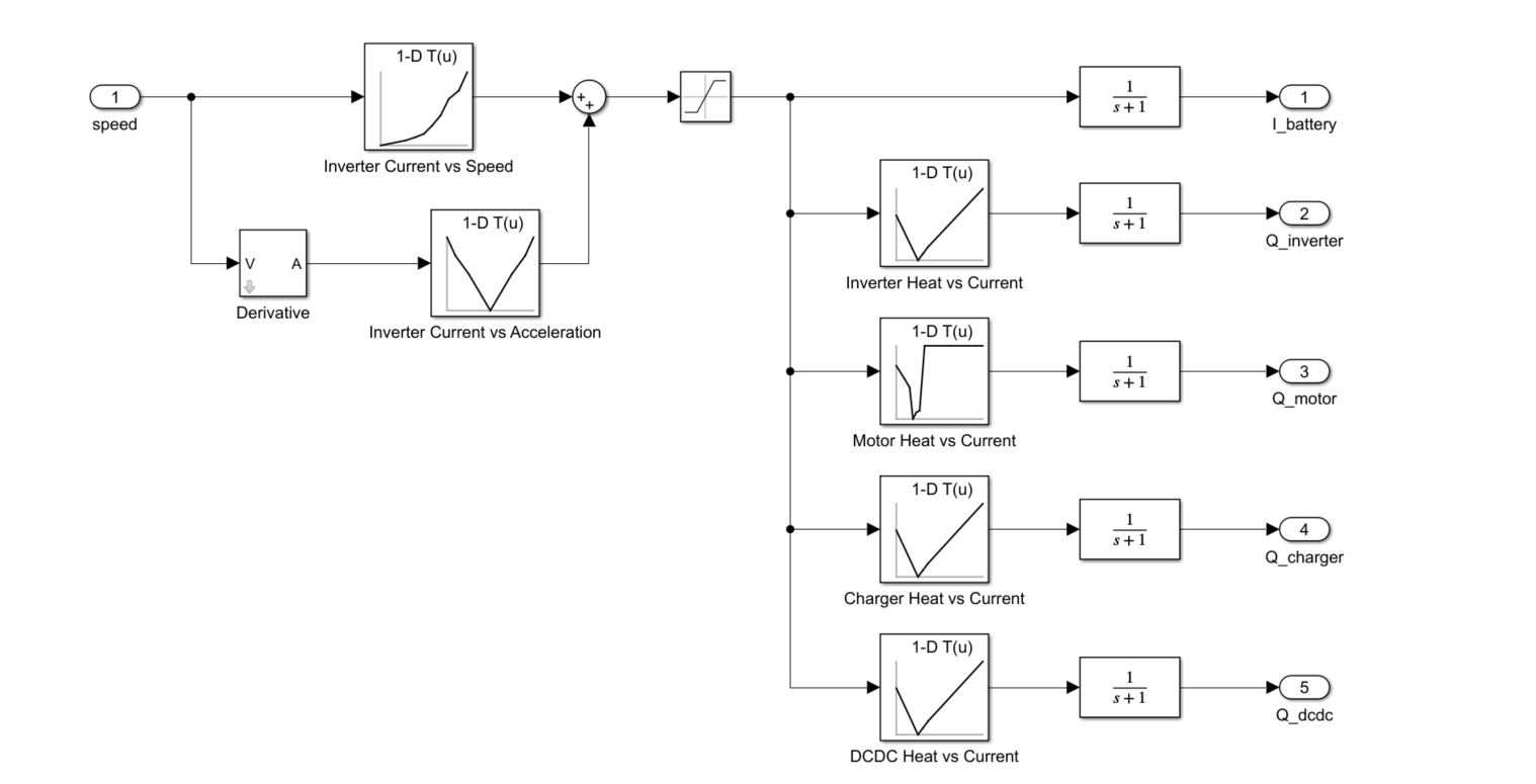
Hello, Recently I have started working on a thermal management project at my Institute. I am taking some hints from en example of EV thermal management provided by MATLAB. I am having an issue in deciding how the battery current and powertrain heat load is calculated as a function of vehicle speed. It would be helpful if someone could provide some links or references regarding this. (Also, attaching a screenshot of the example for better understanding)