結果:
The study of the dynamics of the discrete Klein - Gordon equation (DKG) with friction is given by the equation :

In the above equation, W describes the potential function: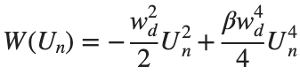
to which every coupled unit  adheres. In Eq. (1), the variable $
 $ is the unknown displacement of the oscillator occupying the n-th position of the lattice, and
  is the discretization parameter. We denote by h the distance between the oscillators of the lattice. The chain (DKG) contains linear damping with a damping coefficient
  , while
 is the coefficient of the nonlinear cubic term.
$ is the unknown displacement of the oscillator occupying the n-th position of the lattice, and For the DKG chain (1), we will consider the problem of initial-boundary values, with initial conditions

and Dirichlet boundary conditions at the boundary points  and
and  , that is,
and , that is,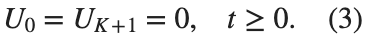
Therefore, when necessary, we will use the short notation  for the one-dimensional discrete Laplacian
for the one-dimensional discrete Laplacian
Now we want to investigate numerically the dynamics of the system (1)-(2)-(3). Our first aim is to conduct a numerical study of the property of Dynamic Stability of the system, which directly depends on the existence and linear stability of the branches of equilibrium points.
For the discussion of numerical results, it is also important to emphasize the role of the parameter  . By changing the time variable
  , we rewrite Eq. (1) in the form
 . We consider spatially extended initial conditions of the form:
We also assume zero initial velocity:
the following graphs for  and
and 
% Parameters
L = 200; % Length of the system
K = 99; % Number of spatial points
j = 2; % Mode number
omega_d = 1; % Characteristic frequency
beta = 1; % Nonlinearity parameter
delta = 0.05; % Damping coefficient
% Spatial grid
h = L / (K + 1);
n = linspace(-L/2, L/2, K+2); % Spatial points
N = length(n);
omegaDScaled = h * omega_d;
deltaScaled = h * delta;
% Time parameters
dt = 1; % Time step
tmax = 3000; % Maximum time
tspan = 0:dt:tmax; % Time vector
% Values of amplitude 'a' to iterate over
a_values = [2, 1.95, 1.9, 1.85, 1.82]; % Modify this array as needed
% Differential equation solver function
function dYdt = odefun(~, Y, N, h, omegaDScaled, deltaScaled, beta)
U = Y(1:N);
Udot = Y(N+1:end);
Uddot = zeros(size(U));
% Laplacian (discrete second derivative)
for k = 2:N-1
Uddot(k) = (U(k+1) - 2 * U(k) + U(k-1)) ;
end
% System of equations
dUdt = Udot;
dUdotdt = Uddot - deltaScaled * Udot + omegaDScaled^2 * (U - beta * U.^3);
% Pack derivatives
dYdt = [dUdt; dUdotdt];
end
% Create a figure for subplots
figure;
% Initial plot
a_init = 2; % Example initial amplitude for the initial condition plot
U0_init = a_init * sin((j * pi * h * n) / L); % Initial displacement
U0_init(1) = 0; % Boundary condition at n = 0
U0_init(end) = 0; % Boundary condition at n = K+1
subplot(3, 2, 1);
plot(n, U0_init, 'r.-', 'LineWidth', 1.5, 'MarkerSize', 10); % Line and marker plot
xlabel('$x_n$', 'Interpreter', 'latex');
ylabel('$U_n$', 'Interpreter', 'latex');
title('$t=0$', 'Interpreter', 'latex');
set(gca, 'FontSize', 12, 'FontName', 'Times');
xlim([-L/2 L/2]);
ylim([-3 3]);
grid on;
% Loop through each value of 'a' and generate the plot
for i = 1:length(a_values)
a = a_values(i);
% Initial conditions
U0 = a * sin((j * pi * h * n) / L); % Initial displacement
U0(1) = 0; % Boundary condition at n = 0
U0(end) = 0; % Boundary condition at n = K+1
Udot0 = zeros(size(U0)); % Initial velocity
% Pack initial conditions
Y0 = [U0, Udot0];
% Solve ODE
opts = odeset('RelTol', 1e-5, 'AbsTol', 1e-6);
[t, Y] = ode45(@(t, Y) odefun(t, Y, N, h, omegaDScaled, deltaScaled, beta), tspan, Y0, opts);
% Extract solutions
U = Y(:, 1:N);
Udot = Y(:, N+1:end);
% Plot final displacement profile
subplot(3, 2, i+1);
plot(n, U(end,:), 'b.-', 'LineWidth', 1.5, 'MarkerSize', 10); % Line and marker plot
xlabel('$x_n$', 'Interpreter', 'latex');
ylabel('$U_n$', 'Interpreter', 'latex');
title(['$t=3000$, $a=', num2str(a), '$'], 'Interpreter', 'latex');
set(gca, 'FontSize', 12, 'FontName', 'Times');
xlim([-L/2 L/2]);
ylim([-2 2]);
grid on;
end
% Adjust layout
set(gcf, 'Position', [100, 100, 1200, 900]); % Adjust figure size as needed
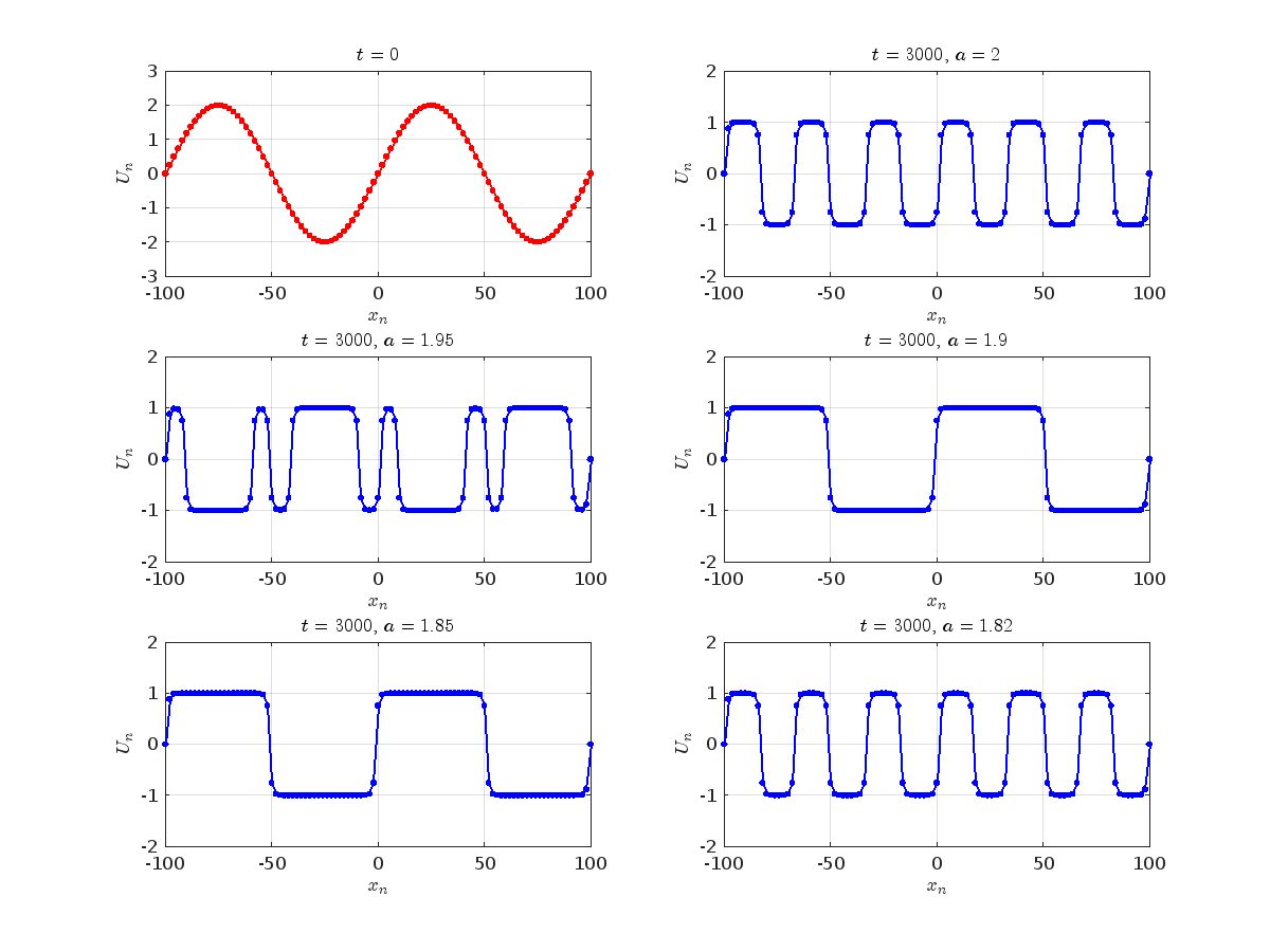
Dynamics for the initial condition ,  , for
, for  , for different amplitude values. By reducing the amplitude values, we observe the convergence to equilibrium points of different branches from
  and the appearance of values
  for which the solution converges to a non-linear equilibrium point
  Parameters:
Detection of a stability threshold  : For
: For  , the initial condition ,
  , converges to a non-linear equilibrium point
 .
.
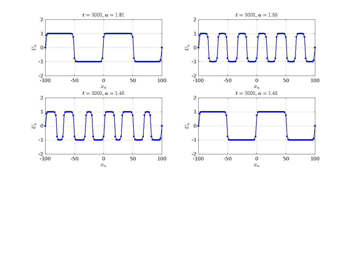
Characteristics for  , with corresponding norm
 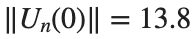 where the dynamics appear in the first image of the third row, we observe convergence to a non-linear equilibrium point of branch
  This has the same norm and the same energy as the previous case but the final state has a completely different profile. This result suggests secondary bifurcations have occurred in branch
where the dynamics appear in the first image of the third row, we observe convergence to a non-linear equilibrium point of branch By further reducing the amplitude, distinct values of  are discerned: 1.9, 1.85, 1.81 for which the initial condition
  with norms
 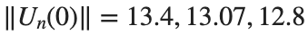 respectively, converges to a non-linear equilibrium point of branch
  This equilibrium point has norm
  and energy
  . The behavior of this equilibrium is illustrated in the third row and in the first image of the third row of Figure 1, and also in the first image of the third row of Figure 2. For all the values between the aforementioned a, the initial condition
  converges to geometrically different non-linear states of branch
  as shown in the second image of the first row and the first image of the second row of Figure 2, for amplitudes
  and
and  respectively.
respectively, converges to a non-linear equilibrium point of branch and energy Refference:
Check out this episode about PIVLab: https://www.buzzsprout.com/2107763/15106425
Join the conversation with William Thielicke, the developer of PIVlab, as he shares insights into the world of particle image velocimetery (PIV) and its applications. Discover how PIV accurately measures fluid velocities, non invasively revolutionising research across the industries. Delve into the development journey of PI lab, including collaborations, key features and future advancements for aerodynamic studies, explore the advanced hardware setups camera technologies, and educational prospects offered by PIVlab, for enhanced fluid velocity measurements. If you are interested in the hardware he speaks of check out the company: Optolution.
One of the starter prompts is about rolling two six-sided dice and plot the results. As a hobby, I create my own board games. I was able to use the dice rolling prompt to show how a simple roll and move game would work. That was a great surprise!
Hallo zusammen,
seit ein paar Tagen werden sämtliche meiner Visualisierungen nicht mehr aktualisiert. Im Editiermodus läuft der Code durch und die Grafik wird korrekt erzeugt.
Hat jemand eine Idee was da schief läuft?
Danke & viele Grüße
Let's talk about probability theory in Matlab.
Conditions of the problem - how many more letters do I need to write to the sales department to get an answer?
To get closer to the problem, I need to buy a license under a contract. Maybe sometimes there are responsible employees sitting here who will give me an answer.
Thank you
In the MATLAB description of the algorithm for Lyapunov exponents, I believe there is ambiguity and misuse.
The lambda(i) in the reference literature signifies the Lyapunov exponent of the entire phase space data after expanding by i time steps, but in the calculation formula provided in the MATLAB help documentation, Y_(i+K) represents the data point at the i-th point in the reconstructed data Y after K steps, and this calculation formula also does not match the calculation code given by MATLAB. I believe there should be some misguidance and misunderstanding here.
According to the symbol regulations in the algorithm description and the MATLAB code, I think the correct formula might be y(i) = 1/dt * 1/N * sum_j( log( ||Y_(j+i) - Y_(j*+i)|| ) )
Cordial saludo , Necesito simular un generador electrico que tiene una entrada mecanica y genera el suficiente voltage y corriente para encender un LED.
Hi Helpdesk,
I urgently seek assistance with an issue that has persisted for a week. I am using Node-RED to interface my gateway and vibration sensor. The sensor sends 960 packets of X, Y, and Z data every 5 minutes. I retrieve and send this data through my Thingspeak42 node to my Thingspeak channel.
I am subscribed to the Thingspeak Student paid plan (see attached "12.png"). Despite this, Thingspeak is inconsistently snipping my data. For example, my X-field sometimes receives only 78 out of 960 points, and similar inconsistencies occur with the Y and Z fields.
Attached is "vibration data node red.png," showing an attempt to send just 120 packets to my Thingspeak channel. However, only 93 data points are received. Also attached is a JSON snapshot of field 2 - X_values, showing only 93 points ("JSON Field 2 data.png"). This is disappointing given that I am paying for the student plan, which should support 33 million points/year per unit (~90,000/day per unit).
I urgently require an explanation and resolution for this issue. Please provide immediate assistance.
Kind regards,
Krish
I have an Arduino Uno R3 with an integrated ESP 8266. With the Arduino Uno, I measure some capacitive humidity sensors and a DHT 22 temperature and humidity sensor. The measurements are sent to the serial port and the ESP 8266 picks them up and uploads them to ThingSpeak. My problem is that it does this randomly and not in the assigned fields. Could someone help me? Thank you very much
Are you local to Boston?
Shape the Future of MATLAB: Join MathWorks' UX Night In-Person!
When: June 25th, 6 to 8 PM
Where: MathWorks Campus in Natick, MA
🌟 Calling All MATLAB Users! Here's your unique chance to influence the next wave of innovations in MATLAB and engineering software. MathWorks invites you to participate in our special after-hours usability studies. Dive deep into the latest MATLAB features, share your valuable feedback, and help us refine our solutions to better meet your needs.
🚀 This Opportunity Is Not to Be Missed:
- Exclusive Hands-On Experience: Be among the first to explore new MATLAB features and capabilities.
- Voice Your Expertise: Share your insights and suggestions directly with MathWorks developers.
- Learn, Discover, and Grow: Expand your MATLAB knowledge and skills through firsthand experience with unreleased features.
- Network Over Dinner: Enjoy a complimentary dinner with fellow MATLAB enthusiasts and the MathWorks team. It's a perfect opportunity to connect, share experiences, and network after work.
- Earn Rewards: Participants will not only contribute to the advancement of MATLAB but will also be compensated for their time. Plus, enjoy special MathWorks swag as a token of our appreciation!
👉 Reserve Your Spot Now: Space is limited for these after-hours sessions. If you're passionate about MATLAB and eager to contribute to its development, we'd love to hear from you.

Hi team,
Could you please confirm us about the process power and computational capacity of ThingSpeak i.e. how quickly and efficiently my MATLAB code can execute on ThingSpeak? What other specifications related to data communication and integration are there in ThingSpeak? As all specifications are not mentioned here: https://thingspeak.com/prices/thingspeak_academic
Thanks.
Regards,
Tanusree
WebSend zu "api.thingspeak.com" zeigt übermittelte Daten an, auf thingspeak kommt aber nichts an.
V11:54:37.665 SCR: performs "WebSend [api.thingspeak.com] /update,json?api_key=***&field1=14039.05&field2=35517.69&field3=-3986.00"
Hat jemand eine Idee warum?
is there any sites available online free ai course learning except: coursera.org
Are you a Simulink user eager to learn how to create apps with App Designer? Or an App Designer enthusiast looking to dive into Simulink?
Don't miss today's article on the Graphics and App Building Blog by @Robert Philbrick! Discover how to build Simulink Apps with App Designer, streamlining control of your simulations!
Northern lights captured from this weekend at MathWorks campus ✨
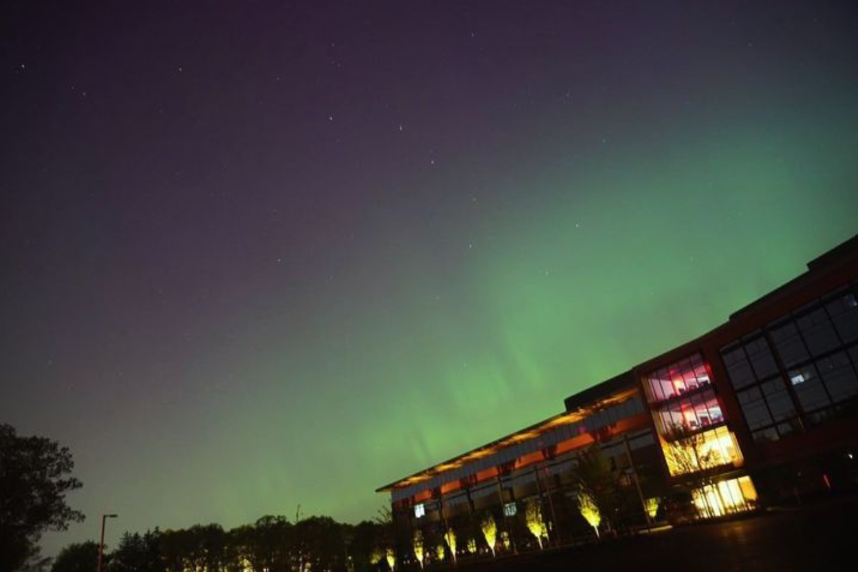
Did you get a chance to see lights and take some photos?
Hi to all.
I'm trying to learn a bit about trading with cryptovalues. At the moment I'm using Freqtrade (in dry-run mode of course) for automatic trading. The tool is written in python and it allows to create custom strategies in python classes and then run them.
I've written some strategy just to learn how to do, but now I'd like to create some interesting algorithm. I've a matlab license, and I'd like to know what are suggested tollboxes for following work:
- Create a criptocurrency strategy algorythm (for buying and selling some crypto like BTC, ETH etc).
- Backtesting the strategy with historical data (I've a bunch of json files with different timeframes, downloaded with freqtrade from binance).
- Optimize the strategy given some parameters (they can be numeric, like ROI, some kind of enumeration, like "selltype" and so on).
- Convert the strategy algorithm in python, so I can use it with Freqtrade without worrying of manually copying formulas and parameters that's error prone.
- I'd like to write both classic algorithm and some deep neural one, that try to find best strategy with little neural network (they should run on my pc with 32gb of ram and a 3080RTX if it can be gpu accelerated).
What do you suggest?
Hi,
I'm a Analysis and systems development student.
Last friday i've created a GPS tracker, using thingspeak api and server, it was working fine until this morning, now it stops.
what could have happened?
i've not even touched the code these days
I isolated a var that I'm interested in, and I want to connect Node-RED to thingspeak to show the values on the graph. The problem is the node "mqttout": I connected it to the server mqtt3.thingspeak.com and the port 1883, and with the device with right username and password. It shows "connected", but the graph is still the same, I can not upload the varabiles.
Dear MATLAB contest enthusiasts,
I believe many of you have been captivated by the innovative entries from Zhaoxu Liu / slanderer, in the 2023 MATLAB Flipbook Mini Hack contest.


Ever wondered about the person behind these creative entries? What drives a MATLAB user to such levels of skill? And what inspired his participation in the contest? We were just as curious as you are!
We were delighted to catch up with him and learn more about his use of MATLAB. The interview has recently been published in MathWorks Blogs. For an in-depth look into his insights and experiences, be sure to read our latest blog post: Community Q&A – Zhaoxu Liu.
But the conversation doesn't end here! Who would you like to see featured in our next interview? Drop their name in the comments section below and let us know who we should reach out to next!
Kindly assist. Im getting this error message when i try to upload to my esp8266 board. I have tried reinstalling arduino ide and libraries. Have also replaced my previous board with a new one.
" fatal esptool.py error occurred: Cannot configure port, something went wrong. Original message: PermissionError(13, 'A device attached to the system is not functioning.', None, 31)esptool.py v3.0
Serial port COM9"