Add Quadrature Mirror and Biorthogonal Wavelet Filters
This example shows how to add an orthogonal quadrature mirror filter (QMF) pair and biorthogonal wavelet filter quadruple to Wavelet Toolbox™. While Wavelet Toolbox™ already contains many orthogonal and biorthogonal wavelet families, you can easily add your own filters and use the filter in any of the discrete wavelet or wavelet packet algorithms.
Add QMF
This section shows how to add a QMF filter pair. Because the example is only for purposes of illustration, you will add a QMF pair that corresponds to a wavelet already available in Wavelet Toolbox™.
Create a vector wavx that contains the scaling filter coefficients for the Daubechies extremal phase wavelet with 2 vanishing moments. You only need a valid scaling filter because the wfilters function creates the corresponding wavelet filter for you.
wavx = [0.482962913145 0.836516303738 0.224143868042 -0.129409522551];
Save the filter and add the new filter to the toolbox. To add to the toolbox an orthogonal wavelet that is defined in a MAT-file, the name of the MAT-file and the variable containing the filter coefficients must match. The name must be less than five characters long.
save wavx wavx
Use wavemngr to add the wavelet filter to the toolbox. Define the wavelet family name and the short name used to access the filter. The short name must be the same name as the MAT-file. Define the wavelet type to be 1. Type 1 wavelets are orthogonal wavelets in the toolbox. Because you are adding only one wavelet in this family, define the NUMS variable input to wavemngr to be an empty string.
familyName      = "Example Wavelet";
familyShortName = "wavx";
familyWaveType  = 1;
familyNums      = "";
fileWaveName    = "wavx.mat";
Add the wavelet using wavemngr.
wavemngr("add",familyName,familyShortName,familyWaveType,familyNums,fileWaveName)Verify that the wavelet has been added to the toolbox.
wavemngr("read")ans = 24×35 char array
'==================================='
'Haar →→haar '
'Daubechies →→db '
'Symlets →→sym '
'Coiflets →→coif '
'BiorSplines →→bior '
'ReverseBior →→rbio '
'Meyer →→meyr '
'DMeyer →→dmey '
'Gaussian →→gaus '
'Mexican_hat →→mexh '
'Morlet →→morl '
'Complex Gaussian →→cgau '
'Shannon →→shan '
'Frequency B-Spline →→fbsp '
'Complex Morlet →→cmor '
'Fejer-Korovkin →→fk '
'Best-localized Daubechies→→bl '
'Morris minimum-bandwidth →→mb '
'Beylkin →→beyl '
'Vaidyanathan →→vaid '
'Han linear-phase moments →→han '
'Example Wavelet →→wavx '
'==================================='
You can now use the wavelet to analyze signals or images. For example, load an ECG signal and obtain the MODWT of the signal down to level four using the new wavelet.
load wecg
wtecg = modwt(wecg,"wavx",4);
Load a box image, obtain the 2-D DWT using the new filter. Show the level-one diagonal detail coefficients.
load xbox
[C,S] = wavedec2(xbox,1,"wavx");
[H,V,D] = detcoef2("all",C,S,1);
subplot(2,1,1)
imagesc(xbox)
axis off
title("Original Image")
subplot(2,1,2)
imagesc(D)
axis off
title("Level-One Diagonal Coefficients")

Obtain the scaling (lowpass) and wavelet (highpass) filters. Use isorthwfb to verify that the filters jointly satisfy the necessary and sufficient conditions to be an orthogonal wavelet filter bank.
[Lo,Hi] = wfilters("wavx");
[tf,checks] = isorthwfb(Lo,Hi)
tf = logical
1
checks=7×3 table
Pass-Fail Maximum Error Test Tolerance
_________ _____________ ______________
Equal-length filters pass 0 0
Even-length filters pass 0 0
Unit-norm filters pass 2.911e-13 1.4901e-08
Filter sums pass 0 1.4901e-08
Even and odd downsampled sums pass 2.2204e-16 1.4901e-08
Zero autocorrelation at even lags pass 2.9092e-13 1.4901e-08
Zero crosscorrelation at even lags pass 5.5511e-17 1.4901e-08
To understand why these filters are called quadrature mirror filters, visualize the squared-magnitude frequency responses of the scaling and wavelet filters.
nfft = 512; F = 0:1/nfft:1/2; LoDFT = fft(Lo,nfft); HiDFT = fft(Hi,nfft); figure plot(F,abs(LoDFT(1:nfft/2+1)).^2) hold on plot(F,abs(HiDFT(1:nfft/2+1)).^2) xlabel("Normalized Frequency") ylabel("Squared Magnitude") title("New QMF Filter Pair") grid on plot([1/4 1/4], [0 2],'k') legend("Scaling Filter","Wavelet Filter") hold off
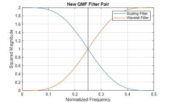
Note the magnitude responses are symmetric, or mirror images, of each other around the quadrature frequency of 1/4.
Remove the new wavelet filter.
wavemngr("del",familyShortName); delete("wavx.mat")
Add Biorthogonal Wavelet
Adding a biorthogonal wavelet to the toolbox is similar to adding a QMF. You provide valid lowpass (scaling) filters pair used in analysis and synthesis. The wfilters function will generate the highpass filters. In this section, you will add the nearly-orthogonal biorthogonal wavelet quadruple based on the Laplacian pyramid scheme of Burt and Adelson (Table 8.4 on page 283 in [1]).
To be recognized by wfilters, the analysis scaling filter must be assigned to the variable Df, and the synthesis scaling filter must be assigned to the variable Rf. The biorthogonal scaling filters do not have to be of even equal length. The output biorthogonal filter pairs created will have even equal lengths. Here are the scaling function pairs of the nearly-orthogonal biorthogonal wavelet quadruple based on the Laplacian pyramid scheme of Burt and Adelson.
Df = [-1 5 12 5 -1]/20*sqrt(2); Rf = [-3 -15 73 170 73 -15 -3]/280*sqrt(2);
Save the filters to a MAT-file.
save burt Df Rf
Use wavemngr to add the biorthogonal wavelet filters to the toolbox. Define the wavelet family name and the short name used to access the filter. The short name must match the name of the MAT-file. Since the wavelets are biorthogonal, set the wavelet type to be 2. Because you are adding only one wavelet in this family, define the NUMS variable input to wavemngr to be an empty string.
familyName = "Burt-Adelson"; familyShortName = "burt"; familyWaveType = 2; familyNums = ""; fileWaveName = "burt.mat"; wavemngr("add",familyName,familyShortName,familyWaveType,familyNums,fileWaveName)
Verify that the biorthogonal wavelet has been added to the toolbox.
wavemngr("read")ans = 24×35 char array
'==================================='
'Haar →→haar '
'Daubechies →→db '
'Symlets →→sym '
'Coiflets →→coif '
'BiorSplines →→bior '
'ReverseBior →→rbio '
'Meyer →→meyr '
'DMeyer →→dmey '
'Gaussian →→gaus '
'Mexican_hat →→mexh '
'Morlet →→morl '
'Complex Gaussian →→cgau '
'Shannon →→shan '
'Frequency B-Spline →→fbsp '
'Complex Morlet →→cmor '
'Fejer-Korovkin →→fk '
'Best-localized Daubechies→→bl '
'Morris minimum-bandwidth →→mb '
'Beylkin →→beyl '
'Vaidyanathan →→vaid '
'Han linear-phase moments →→han '
'Burt-Adelson →→burt '
'==================================='
You can now use the wavelet within the toolbox.
Obtain the lowpass and highpass analysis and synthesis filters associated with the burt wavelet. Note the output filters are of equal even length.
[LoD,HiD,LoR,HiR] = wfilters("burt");
[LoD' HiD' LoR' HiR']ans = 8×4
0 0.0152 -0.0152 0
0 -0.0758 -0.0758 0
-0.0707 -0.3687 0.3687 -0.0707
0.3536 0.8586 0.8586 -0.3536
0.8485 -0.3687 0.3687 0.8485
0.3536 -0.0758 -0.0758 -0.3536
-0.0707 0.0152 -0.0152 -0.0707
0 0 0 0
Use isbiorthwfb to confirm the four filters jointly satisfy the necessary and sufficient conditions to be a two-channel biorthogonal perfect reconstruction wavelet filter bank.
[tf,checks] = isbiorthwfb(LoR,LoD,HiR,HiD)
tf = logical
   1
checks=7×3 table
                                                       Pass-Fail    Maximum Error    Test Tolerance
                                                       _________    _____________    ______________

    Dual filter lengths correct                          pass                 0                 0
    Filter sums                                          pass        2.2204e-16        1.4901e-08
    Zero lag lowpass dual filter cross-correlation       pass        2.2204e-16        1.4901e-08
    Zero lag highpass dual filter cross-correlation      pass                 0        1.4901e-08
    Even lag lowpass dual filter cross-correlation       pass        1.7347e-18        1.4901e-08
    Even lag highpass dual filter cross-correlation      pass        2.7756e-17        1.4901e-08
    Even lag lowpass-highpass cross-correlation          pass        6.9389e-18        1.4901e-08
Create an analysis DWT filter bank using the burt wavelet. Plot the magnitude frequency responses of the wavelet bandpass filters and coarsest resolution scaling function.
fb = dwtfilterbank(Wavelet="burt");
freqz(fb)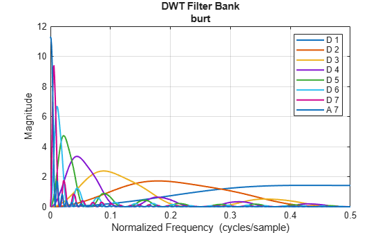
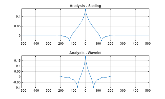
Obtain the wavelet and scaling functions of the filter bank. Plot the wavelet and scaling functions at the coarsest scale.
[fb_phi,t] = scalingfunctions(fb);
[fb_psi,~] = wavelets(fb);
subplot(2,1,1)
plot(t,fb_phi(end,:))
axis tight
grid on
title("Analysis - Scaling")
subplot(2,1,2)
plot(t,fb_psi(end,:))
axis tight
grid on
title("Analysis - Wavelet")
Create a synthesis DWT filter bank using the burt wavelet. Compute the framebounds.
fb2 = dwtfilterbank(Wavelet="burt",FilterType="Synthesis",Level=4);
[synthesisLowerBound,synthesisUpperBound] = framebounds(fb2)
synthesisLowerBound =
0.9800
synthesisUpperBound =
1.0509
Remove the Burt-Adelson filter from the Toolbox.
wavemngr("del",familyShortName);
delete("burt.mat")
References
[1] Daubechies, I. Ten Lectures on Wavelets. CBMS-NSF Regional Conference Series in Applied Mathematics. Philadelphia, PA: Society for Industrial and Applied Mathematics, 1992.
See Also
waveinfo | wavemngr | wfilters | isorthwfb | isbiorthwfb