cqt

Constant-Q nonstationary Gabor transform

Syntax

cfs = cqt(x)

[cfs,f] = cqt(x)

[cfs,f,g,fshifts] = cqt(x)

[cfs,f,g,fshifts,fintervals] = cqt(x)

[cfs,f,g,fshifts,fintervals,bw] = cqt(x)

[___] = cqt(___,Name,Value)

cqt(___)

Description

cfs = cqt(x) returns the constant-Q transform (CQT), cfs, of the input signal x. The input signal must have at least four samples.

• If x is a vector, then cqt returns a matrix corresponding to the CQT.

• If x is a matrix, then cqt obtains the CQT for each column (independent channel) of x. The function returns a multidimensional array corresponding to the maximally redundant version of the CQT.

[cfs,f] = cqt(x) returns the approximate bandpass center frequencies, f, corresponding to the rows of cfs. The frequencies are ordered from 0 to 1 and are in cycles/sample.

[cfs,f,g,fshifts] = cqt(x) returns the Gabor frames, g, used in the analysis of x and the frequency shifts, fshifts, in discrete Fourier transform (DFT) bins between the passbands in the rows of cfs.

cfs, g, and fshifts are required inputs for the inversion of the CQT with icqt.

[cfs,f,g,fshifts,fintervals] = cqt(x) returns the frequency intervals, fintervals, corresponding the rows of cfs. The kth element of fshifts is the frequency shift in DFT bins between the ((k-1) mod N) and (k mod N) element of fintervals with k = 0,1,2,...,N-1, where N is the number of frequency shifts. Because MATLAB^® indexes from 1, fshifts(1) contains the frequency shift between fintervals{end} and fintervals{1}, fshifts(2) contains the frequency shift between fintervals{1} and fintervals{2}, and so on.

[cfs,f,g,fshifts,fintervals,bw] = cqt(x) returns the bandwidth, bw, in DFT bins of the frequency intervals, fintervals.

[___] = cqt(___,Name,Value) returns the CQT with additional options specified by one or more Name,Value pair arguments, using any of the preceding syntaxes.

cqt(___) with no output arguments plots the CQT in the current figure. Plotting is supported for vector inputs only. If the input signal is real and Fs is the sampling frequency, the CQT is plotted over the range [0,Fs/2]. If the signal is complex, the CQT is plotted over the range [0,Fs).

Note

In order to visualize a sparse CQT, coefficients have to be interpolated. When interpolation occurs, the plot can have significant smearing and be difficult to interpret. If you want to plot the CQT, we recommend using the default TransformType value 'full'.

Examples

Constant-Q Transform Using Default Values

Load a signal and obtain the constant-Q transform.

load noisdopp
cfs = cqt(noisdopp);

Center Frequencies of the Constant-Q Transform

Load a real-valued signal and obtain the constant-Q transform. Return the approximate bandpass center frequencies.

load handel
[cfs,f] = cqt(y);

Plot on a logarithmic scale the bandpass center frequencies through the Nyquist frequency.

lfreq = length(f);
nyquistBin = floor(lfreq/2)+1;
plot(f(1:nyquistBin))
title('Bandpass Center Frequencies')
grid on
set(gca,'yscale','log')

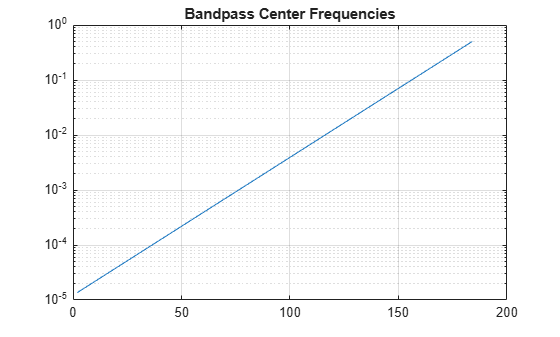
By default, cqt uses 12 bins per octave. Confirm the ratios of consecutive pairs of frequencies are approximately equal to $$2^{1/12}$$. Since the DC and Nyquist frequencies are not members of the geometric sequence of center frequencies, exclude them from the frequency vector.

geoRatio = f(3:nyquistBin-1)./f(2:nyquistBin-2);
[2^(1/12) min(geoRatio) max(geoRatio)]

ans = 1×3

    1.0595    1.0595    1.0595

Visualize and Apply Constant-Q Transform Gabor Frames

Obtain the minimally redundant constant-Q transform of an audio signal. Use the Blackman-Harris window as the prototype function for the Gabor frames.

load handel
df = Fs/numel(y);
[cfs,f,g,fshifts,fintervals,bw] = cqt(y,'SamplingFrequency',Fs, ...
    'TransformType',"sparse",...
    'Window',"blackmanharris");

cfs is a cell array, where each element in the array corresponds to a bandpass center frequency and Gabor frame. Plot the Gabor frame associated with the Nyquist frequency.

lf = length(f);
ind = floor(lf/2)+1;
gFrame = fftshift(g{ind});
fvec = f(ind-1):df:f(ind+1)-df;
plot(fvec,gFrame)
xlabel('Frequency (Hz)')
grid on
title({"Gabor Frame - Freq: "+num2str(f(ind))+" Hz", ...
    "Bandwidth: "+num2str(bw(ind)*Fs/numel(y))+" Hz"})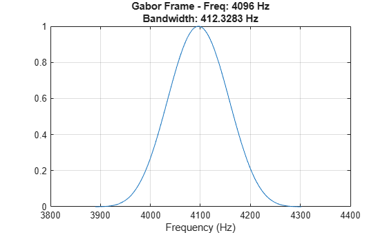

In the constant-Q transform, the Gabor frames are applied to the discrete Fourier transform of the input signal, and the inverse discrete Fourier transform is performed. The kth Gabor frame is applied to the kth frequency interval specified in fintervals. Take the discrete Fourier transform of the signal and plot its magnitude spectrum. Use fintervals to indicate over which Fourier coefficients are the Gabor frame associated with the Nyquist frequency are applied.

yDFT = fft(y);
lyDFT = length(yDFT);
plot(Fs*(0:lyDFT-1)/lyDFT,abs(yDFT))
grid on
fIntervalGabor = fintervals{ind};
mx = max(abs(yDFT));
hold on
plot([df*fIntervalGabor(1) df*fIntervalGabor(1)],[0 mx], ...
    'r-','LineWidth',2)
plot([df*fIntervalGabor(end) df*fIntervalGabor(end)],[0 mx], ...
    'r-','LineWidth',2)
str = sprintf('Gabor Frame Interval (Hz): [%3.2f, %3.2f]', ...
    df*fIntervalGabor(1),df*fIntervalGabor(end));
title(str)
xlabel('Frequency (Hz)')
ylabel('Magnitude')

Window the Fourier coefficients in the interval with the Gabor frame, and take the inverse discrete Fourier transform. Normalize the result, and compare with computed constant-Q coefficients and confirm they are equal.

lGframe = length(gFrame);
indx = 1:lGframe;
indx = fftshift(indx);
winDFT(indx) = yDFT(fIntervalGabor).*fftshift(gFrame(indx));
cqCoefs = ifft(winDFT);
cqCoefs = (2*lGframe/length(y))*cqCoefs;
max(abs(cqCoefs(:)-cfs{ind}(:)))

ans = 
0

Constant-Q Transform of Audio Signal

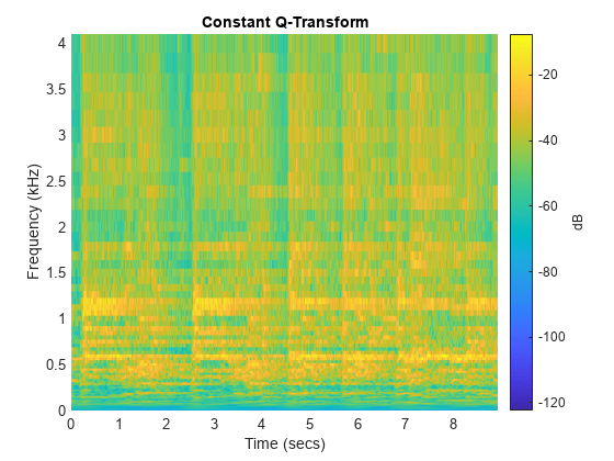
Load an audio signal. Plot the constant-Q transform (CQT) using the maximally redundant version of the transform and using 12 bins per octave.

load handel
cqt(y,'SamplingFrequency',Fs)

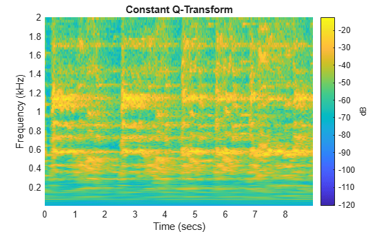
Obtain the CQT of the signal using 48 bins per octave. Set the frequency range from the smallest allowable center frequency to 2 kHz.

minFreq = Fs/length(y);
maxFreq = 2000;
figure
cqt(y,'SamplingFrequency',Fs, ...
    'BinsPerOctave',48, ...
    'FrequencyLimits',[minFreq maxFreq])

Input Arguments

x — Input signal

vector | matrix

Input signal, specified as a real or complex vector or matrix. x must have at least four samples.

Data Types: double
Complex Number Support: Yes

Name-Value Arguments

Specify optional pairs of arguments as Name1=Value1,...,NameN=ValueN, where Name is the argument name and Value is the corresponding value. Name-value arguments must appear after other arguments, but the order of the pairs does not matter.

Before R2021a, use commas to separate each name and value, and enclose Name in quotes.

Example: 'SamplingFrequency',20,'BinsPerOctave',15

SamplingFrequency — Sampling frequency

positive scalar

Sampling frequency, in Hz, specified as the comma-separated pair consisting of 'SamplingFrequency' and a positive scalar.

BinsPerOctave — Number of bins per octave

12 (default) | positive integer from 1 to 96

Number of bins per octave to use in the CQT, specified as a positive integer from 1 to 96.

TransformType — Type of constant-Q transform

'full' (default) | 'sparse'

Type of constant-Q transform to perform, specified as the comma-separated pair consisting of 'TransformType' and 'full' or 'sparse'. The sparse transform is the minimally redundant version of the constant-Q transform.

FrequencyLimits — Frequency limits

two-element real vector

Frequency limits over which the CQT has a logarithmic frequency response with the specified number of frequency bins per octave, specified as the comma-separated pair 'FrequencyLimits' and a two-element real vector.

• The first element must be greater than or equal to Fs/N, where Fs is the sampling frequency and N is the length of the signal.

• The second element must be strictly less than the Nyquist frequency.

Window — Window to use as prototype function

'hann' (default) | 'hamming' | 'blackmanharris' | 'itersine' | 'bartlett'

Window to use as the prototype function for the nonstationary Gabor frames, specified as 'hann', 'hamming', 'blackmanharris', 'itersine', or 'bartlett'. These compactly support functions are defined in frequency. For normalized frequencies, they are defined on the interval (-1/2,1/2). If you specify a sampling frequency, Fs, they are defined on the interval (-Fs/2,Fs/2).

Output Arguments

cfs — Constant-Q transform

matrix | multidimensional array | cell array | structure array

Constant-Q transform, returned as a matrix, multidimensional array, cell array, or structure array.

• If 'TransformType' is specified as 'full' without 'FrequencyLimits', cfs is a matrix or multidimensional array.

  • If x is a vector, then cqt returns a matrix corresponding to the CQT.

  • If x is a matrix, then cqt obtains the CQT for each column (independent channel) of x. The function returns a multidimensional array corresponding to the maximally redundant version of the CQT.

  The array, cfs, corresponds to the maximally redundant version of the CQT. Each row of the pages of cfs corresponds to passbands with normalized center frequencies (cycles/sample) logarithmically spaced between 0 and 1. A normalized frequency of 1/2 corresponds to the Nyquist frequency. The number of columns, or hops, corresponds to the largest bandwidth center frequency, which usually occurs one frequency bin below or above the Nyquist bin.

• If 'TransformType' is specified as 'full' and you specify frequency limits, cfs is returned as a structure array with the following four fields.

  • c — Coefficient matrix of multidimensional array for the frequencies within the specified frequency limits. This includes both the positive and "negative" frequencies.

  • DCcfs — Coefficient vector or matrix for the passband from 0 to the lower frequency limit.

  • Nyquistcfs — Coefficient vector or matrix for the passband from the upper frequency limit to the Nyquist.

  • NyquistBin — DFT bin corresponding to the Nyquist frequency. This field is used when inverting the CQT.

• If 'TransformType' is specified as 'sparse', cfs is a cell array with the number of elements equal to the number of bandpass frequencies. Each element of the cell array, cfs, is a vector or matrix with the number of rows equal to the value of the bandwidth in DFT bins, bw.

cfs, g, and fshifts are required inputs for the inversion of the CQT with icqt.

f — Approximate bandpass center frequencies

real-valued vector

Approximate bandpass center frequencies corresponding to the rows of cfs, returned as a real-valued vector. The frequencies are ordered from 0 to 1 and are in cycles/sample. If you specified 'SamplingFrequency', then f is in Hertz.

g — Gabor frames

cell array of real-valued vectors

Gabor frames used in the analysis of x, returned as a cell array of real-valued vectors. Each vector in g corresponds to a row of cfs.

cfs, g, and fshifts are required inputs for the inversion of the CQT with icqt.

fshifts — Frequency shifts

real-valued vector

Frequency shifts in discrete Fourier transform bins, returned as a real-valued vector. The shifts are between the passbands in the rows of cfs.

cfs, g, and fshifts are required inputs for the inversion of the CQT with icqt.

fintervals — Frequency intervals

cell array of real-valued vectors

Frequency intervals corresponding to the rows of cfs, returned as a cell array. Each element in fintervals is a real-valued vector. The kth element of fshifts is the frequency shift in DFT bins between the ((k-1) mod N) and (k mod N) element of fintervals with k = 0,1,2,...,N-1 where N is the number of frequency shifts. Because MATLAB indexes from 1, fshifts(1) contains the frequency shift between fintervals{end} and fintervals{1}, fshifts(2) contains the frequency shift between fintervals{1} and fintervals{2}, and so on.

bw — Bandwidths

real-valued vector

Bandwidths in DFT bins of the frequency intervals, fintervals, returned as a real-valued vector.

Algorithms

Nonstationary Gabor Frames

The theory of nonstationary Gabor transforms (NSGTs) was introduced by Jaillet [1] and Balazs, Dörfler, Jaillet, Holighaus, and Velasco [2]. Dörfler, Holighaus, Grill, and Velasco [3], [4] develop a framework for an efficient, perfectly invertible CQT. The algorithms used in cqt and icqt were developed by Dörfler, Holighaus, Grill, and Velasco and are described in [3], [4]. In [5], Schörkhuber, Klapuri, Holighaus, and Dörfler develop and provide algorithms for a phase-corrected CQT transform which matches the CQT coefficients that would be obtained by naïve convolution. The Large Time-Frequency Analysis Toolbox (https://github.com/ltfat) provides an extensive suite of algorithms for nonstationary Gabor frames [6].

Perfect Reconstruction

To achieve the perfect reconstruction property of the constant-Q analysis with nonstationary Gabor frames, cqt internally prepends the zero frequency (DC) and appends the Nyquist frequency to the frequency interval. The negative frequencies are mirrored versions of the positive center frequencies and bandwidths

References

[1] Jaillet, Florent. “Représentation et traitement temps-fréquence des signaux audionumériques pour des applications de design sonore.” Ph.D. dissertation, Université de la Méditerranée, Aix-Marseille II, 2005.

[2] Balazs, P., M. Dörfler, F. Jaillet, N. Holighaus, and G. Velasco. “Theory, Implementation and Applications of Nonstationary Gabor Frames.” Journal of Computational and Applied Mathematics 236, no. 6 (October 2011): 1481–96. https://doi.org/10.1016/j.cam.2011.09.011.

[3] Holighaus, Nicki, M. Dörfler, G. A. Velasco, and T. Grill. “A Framework for Invertible, Real-Time Constant-Q Transforms.” IEEE Transactions on Audio, Speech, and Language Processing 21, no. 4 (April 2013): 775–85. https://doi.org/10.1109/TASL.2012.2234114.

[4] Velasco, G. A., N. Holighaus, M. Dörfler, and T. Grill. "Constructing an invertible constant-Q transform with nonstationary Gabor frames." In Proceedings of the 14th International Conference on Digital Audio Effects (DAFx-11). Paris, France: 2011.

[5] Schörkhuber, C., A. Klapuri, N. Holighaus, and M. Dörfler. "A MATLAB Toolbox for Efficient Perfect Reconstruction Time-Frequency Transforms with Log-Frequency Resolution." Submitted to the AES 53rd International Conference on Semantic Audio. London, UK: 2014.

[6] Průša, Z., P. L. Søndergaard, N. Holighaus, C. Wiesmeyr, and P. Balazs. The Large Time-Frequency Analysis Toolbox 2.0. Sound, Music, and Motion, Lecture Notes in Computer Science 2014, pp 419-442.

Extended Capabilities

C/C++ Code Generation

Generate C and C++ code using MATLAB® Coder™.

Usage notes and limitations:

• The value of the 'TransformType' name-value pair argument must be constant. Use coder.Constant.

• Plotting is not supported.

Version History

Introduced in R2018a