Finite Element Formulation for Timoshenko Beam Problem

This example shows how to apply the finite element method (FEM) to solve a Timoshenko beam problem, using both linear and quadratic basis functions for analysis. The Timoshenko beam theory is a 1-D problem that reduces the complex 3-D problem of beam deformation to a set of 1-D differential equations along the length of the beam. In contrast to the Euler–Bernoulli beam theory, which does not consider shear deformation, the Timoshenko beam theory accounts for both shear deformation and rotational bending effects. The Timoshenko beam theory is generally more accurate for short, thick beams where shear deformation cannot be neglected. Using a cantilever beam and a beam fixed at both ends, this example discusses the analytical solutions of the Timoshenko beam problem and compares them with the FEM solutions.

In the thin beam limit of the standard variational formulation, the Timoshenko beam model becomes susceptible to the transverse shear locking effect. The term locking refers to an artificial stiffening, as if the beam's cross sections are "locked" together and unable to shear properly relative to each other. This issue is more pronounced when using lower-order basis functions in the FEM analysis. This example compares the results derived from linear basis functions and from quadratic basis functions to illustrate how using higher-order functions reduces the locking effect in the Timoshenko beam analysis.

Define Beam Parameters

In this example, the Timoshenko beam extends along the $$x$$-axis, with vertical displacement $$w(x)$$ in the transversal direction along the $$z$$-axis and bending rotation angle $$\beta (x)$$ with rotation around the $$y$$-axis.

First, define the geometrical parameters of the beam and set their values in SI units.

• $$t$$ is thickness of the beam, in m.

• $$b$$ is the width of the beam, in m.

• $$A$$ is the cross-sectional area of the beam, in m².

• $$L$$ is the length of the beam, in m. The left-end x-coordinate of the beam is at 0, so $$L$$ also corresponds to the right-end x-coordinate of the beam.

beamParams.t = 10^-2;
beamParams.b = 0.1;
beamParams.A = beamParams.b*beamParams.t;
beamParams.L = 4;

Next, define the load and material parameters of the beam and set their values in SI units.

• $\bar{\mathit{q}}$ is the external transversal distributed load along the beam's length, in N/m. The load value is set to be proportional to the thickness of the beam to the power of 3 and constant along the $$x$$-axis.

• $\bar{\mathit{m}}$ is the external distributed bending moment along the beam's length, in N. The moment is set to 0.

• $$E$$ is Young's modulus, in N/m².

• $$\nu$$ is Poisson's ratio.

• $$I$$ is the moment of inertia of the beam's rectangular cross section in the$$yz$$-plane, in m⁴. Here, assume you scale the model to represent a uniform mass distribution across the beam, where the mass per area equals 1 and the moment of inertia is $$I=b{t}^3/12$$.

• $$G$$ is the shear modulus, in N/m².

• $$\alpha$$ is the shear correction factor. This parameter accounts for the cross section of the beam not always being planar in the $$yz$$-plane nor remaining orthogonal to the tangent of the beam axis due to bending.

beamParams.q_bar = -(beamParams.t)^3;
beamParams.m_bar = 0;
beamParams.E = 1e7;
beamParams.nu = 0.3;
beamParams.I = beamParams.b*(beamParams.t^3)/12;
beamParams.G = beamParams.E/(2*(1 + beamParams.nu));
beamParams.alpha = 5/6;

Unlike the Euler-Bernoulli beam theory, which assumes that plane sections remain plane and perpendicular to the neutral axis, the Timoshenko beam theory accounts for shear deformation. This means that the cross-sections can warp, and the bending rotation angle $$\beta (x)$$ is not necessarily the same as the slope of the deflection curve. For small angle approximations and an external load applied downward in the $$-z$$ direction, the angle of the deflection curve is $$-dw(x)/dx$$. The shear angle $$\gamma (x)$$ can be obtained as the difference between the bending rotation angle and the angle of the deflection curve, that is

$\gamma \left(\mathit{x}\right)=\beta \left(\mathit{x}\right)-\left(-\frac{\mathit{dw}\left(\mathit{x}\right)}{\mathit{dx}}\right)=\beta \left(\mathit{x}\right)+\frac{\mathit{dw}\left(\mathit{x}\right)}{\mathit{dx}}.$

Derive Equilibrium Equations for Timoshenko Beam

The Timoshenko beam theory introduces two variables: the transverse deflection $$w(x)$$ along the $$z$$-axis and the bending rotation angle $$\beta (x)$$ with respect to the $$y$$-axis. These variables as a function of $$x$$, or the beam axial direction, describe the displacements of the beam under external load and bending moment. The theory further relates the internal load and moment through constitutive laws based on the material properties, leading to a set of equilibrium equations for the beam.

From the two displacement fields $$w(x)$$ and $$\beta (x)$$, define the shear angle $$\gamma (x)$$ and the bending curvature $$\kappa (x)$$.

$$\begin{array}{l}\gamma \left(\mathit{x}\right)=\beta \left(\mathit{x}\right)+\frac{\mathit{dw}\left(\mathit{x}\right)}{\mathit{dx}},\\ \kappa \left(\mathit{x}\right)=\frac{\mathit{d}\beta \left(\mathit{x}\right)}{\mathit{dx}}.\end{array}$$

The constitutive laws, according to Hooke's laws that relate the stresses to strains, lead to these equations for the internal load (or the internal shear force) $$Q(x)$$ and the internal moment $$M(x)$$.

$$\begin{array}{l}\mathit{Q}\left(\mathit{x}\right)=\alpha \mathit{GA}\gamma \left(\mathit{x}\right),\\ \mathit{M}\left(\mathit{x}\right)=\mathit{EI}\kappa \left(\mathit{x}\right).\end{array}$$

With the presence of an external distributed moment $$m(x)$$ and external distributed force $$q(x)$$, the equilibrium equations of the Timoshenko beam, according to Newton's laws, are:

$$\begin{array}{l}-\frac{\mathit{dM}}{\mathit{dx}}+\mathit{Q}=\mathit{m}\left(\mathit{x}\right),\\ -\frac{\mathit{dQ}}{\mathit{dx}}=\mathit{q}\left(\mathit{x}\right).\end{array}$$

In terms of the displacement variables $$w$$ and $$\beta$$, the equilibrium equations become:

$$-\frac{\mathit{d}}{\mathit{dx}}\left(\mathit{EI}\frac{\mathit{d}\beta }{\mathit{dx}}\right)+\alpha \mathit{GA}\left(\beta +\frac{\mathit{dw}}{\mathit{dx}}\right)=\mathit{m}\left(\mathit{x}\right),$$	(1)
$$-\frac{\mathit{d}}{\mathit{dx}}\left(\alpha \mathit{GA}\left(\beta +\frac{\mathit{dw}}{\mathit{dx}}\right)\right)=\mathit{q}\left(\mathit{x}\right).$$	(2)

Find Analytical Solution for Cantilever Beam Fixed at One End

Consider a cantilever beam that is fixed at one end and free at the other. When an external uniformly distributed load $$\underset{}{\overset{‾}{q}}$$ is applied to the cantilever beam, the beam displacements $$w(x)$$ and $$\beta (x)$$ have analytical solutions. You can use Symbolic Math Toolbox™ to derive these analytical solutions from the equilibrium equations by applying the necessary boundary conditions.

Create the symbolic variables for the displacement variables and the beam parameters.

syms w(x) beta(x) A L q_bar m_bar E I G alpha

Define the equilibrium equations by setting the external load and the external moment as $$q(x)=\underset{}{\overset{‾}{q}}$$ and $$m(x)=0$$, respectively.

Q = alpha*G*A*(beta + diff(w,x));
M = E*I*diff(beta,x);
eqns = [-diff(M,x) + Q == 0;
        -diff(Q,x) == q_bar]

eqns(x) = 
$$\left(\begin{array}{c}A\hspace{0.17em}G\hspace{0.17em}\alpha \hspace{0.17em}\left(\frac{\partial }{\partial x}\mathrm{ }w\left(x\right)+\beta \left(x\right)\right)-\text{E}\hspace{0.17em}\text{I}\hspace{0.17em}\frac{{\partial }^2}{\partial x^2}\mathrm{ }\beta \left(x\right)=0\\ -A\hspace{0.17em}G\hspace{0.17em}\alpha \hspace{0.17em}\left(\frac{{\partial }^2}{\partial x^2}\mathrm{ }w\left(x\right)+\frac{\partial }{\partial x}\mathrm{ }\beta \left(x\right)\right)=\bar{q}\end{array}\right)$$

The boundary conditions for a fixed left end of the cantilever beam are $$w(0)=0$$ and $$\beta (0)=0$$. Meanwhile, the boundary conditions for the free right end of the beam are $$\gamma (L)=0$$ and $$\kappa (L)=0$$, or equivalently $$Q(L)=M(L)=0$$. Define these boundary conditions by introducing the intermediary variables for $$dw/dx$$ and $$d\beta /dx$$ that follow the definition of $$\gamma$$ and $$\kappa$$.

Dw(x) = diff(w,x);
Dbeta(x) = diff(beta,x);
cond = [w(0)==0; beta(0)==0; beta(L)==-Dw(L); Dbeta(L)==0];

Find the analytical solutions for $$w(x)$$ and $$\beta (x)$$ by using dsolve on the equilibrium equations and the specified boundary conditions. Simplify the solutions by using simplify.

[beta_sol,w_sol] = dsolve(eqns,cond);
w_sol = simplify(w_sol)

w_sol = 
$$\frac{\bar{q}\hspace{0.17em}x\hspace{0.17em}\left(6\hspace{0.17em}A\hspace{0.17em}G\hspace{0.17em}\alpha \hspace{0.17em}{L}^2\hspace{0.17em}x-4\hspace{0.17em}A\hspace{0.17em}G\hspace{0.17em}\alpha \hspace{0.17em}L\hspace{0.17em}{x}^2+24\hspace{0.17em}\text{E}\hspace{0.17em}\text{I}\hspace{0.17em}L+A\hspace{0.17em}G\hspace{0.17em}\alpha \hspace{0.17em}{x}^3-12\hspace{0.17em}\text{E}\hspace{0.17em}\text{I}\hspace{0.17em}x\right)}{24\hspace{0.17em}A\hspace{0.17em}\text{E}\hspace{0.17em}G\hspace{0.17em}\text{I}\hspace{0.17em}\alpha }$$

beta_sol = simplify(beta_sol)

beta_sol = 
$$-\frac{\bar{q}\hspace{0.17em}x\hspace{0.17em}\left(3\hspace{0.17em}{L}^2-3\hspace{0.17em}L\hspace{0.17em}x+x^2\right)}{6\hspace{0.17em}\text{E}\hspace{0.17em}\text{I}}$$

Most textbooks on structural analysis include solutions for cantilever beam displacements. For comparison, define the solutions from references [1] and [2]. Compare the textbook solutions with the analytical solutions obtained using Symbolic Math Toolbox by using isAlways. The results are logical 1, meaning that the textbook solutions agree with the solutions returned by dsolve.

w_ref(x) = 1/(alpha*G*A)*(q_bar*L*x - q_bar*x^2/2) - ...
    1/(E*I)*(-q_bar*x^4/24 + q_bar*L*x^3/6 - q_bar*L^2*x^2/4)

w_ref(x) = 
$$\frac{\frac{\bar{q}\hspace{0.17em}{L}^2\hspace{0.17em}{x}^2}{4}-\frac{\bar{q}\hspace{0.17em}L\hspace{0.17em}{x}^3}{6}+\frac{\bar{q}\hspace{0.17em}{x}^4}{24}}{\text{E}\hspace{0.17em}\text{I}}-\frac{\frac{\bar{q}\hspace{0.17em}{x}^2}{2}-L\hspace{0.17em}\bar{q}\hspace{0.17em}x}{A\hspace{0.17em}G\hspace{0.17em}\alpha }$$

syms x_a
beta_ref(x) = int(-q_bar/(alpha*G*A) - diff(w_ref(x_a),2),x_a,0,x)

beta_ref(x) = 
$$-\frac{\bar{q}\hspace{0.17em}x\hspace{0.17em}\left(3\hspace{0.17em}{L}^2-3\hspace{0.17em}L\hspace{0.17em}x+x^2\right)}{6\hspace{0.17em}\text{E}\hspace{0.17em}\text{I}}$$

tf_w = isAlways(w_ref == w_sol)

tf_w = logical
   1

tf_beta = isAlways(beta_ref == beta_sol)

tf_beta = logical
   1

Next, modify the analytical solutions by substituting the values of all known parameters of the beam. In the next sections, you will plot these analytical solutions and compare them with the FEM solutions.

w_eval = subs(w_sol,beamParams);
beta_eval = subs(beta_sol,beamParams);

Implement Basis Interpolation Functions for FEM

The FEM is a numerical technique used to solve complex engineering and mathematical problems by breaking them down into smaller, simpler parts called finite elements. These elements are interconnected at points known as nodes, forming a mesh that approximates the geometry of the original system. By discretizing the domain into a finite number of elements, FEM transforms a complex problem into a set of algebraic equations that can be solved computationally. Each element is governed by simplified equations that approximate the system's behavior, and these local equations are assembled into a global system.

In the FEM formulation of the Timoshenko beam, the displacement fields $$w^i$$ and $${\beta }^i$$ on each mesh element, indexed by $$i$$, are approximated using basis interpolation functions. These basis functions are defined in terms of the discretized nodal values and the shape functions. One method to define the shape functions is through the use of Lagrange polynomials. To incorporate an isoparametric representation of the problem, which accommodates both constant and linear strain states of the mesh elements, the same shape functions are used to define both the element's geometric shape and the displacement fields. Consequently, this example defines the displacements $$w^i$$, $${\beta }^i$$, and the global coordinate $$x^i$$ of each element as functions of the local coordinate $$\xi$$ using the same shape functions, where:

$$\begin{array}{l}{\mathit{w}}^{\mathit{i}}\left(\xi \right)\approx \sum _{\mathit{j}=1}^{\mathit{m}}{\mathit{N}}_{\mathit{j}}\left(\xi \right){{\mathit{w}}^{\mathit{i}}}_{\mathit{j}},\\ {\beta }^{\mathit{i}}\left(\xi \right)\approx \sum _{\mathit{j}=\mathrm{1}}^{\mathit{m}}{\mathit{N}}_{\mathit{j}}\left(\xi \right){{\beta }^{\mathit{i}}}_{\mathit{j}},\\ {\mathit{x}}^{\mathit{i}}\left(\xi \right)=\sum _{\mathit{j}=1}^{\mathit{m}}{\mathit{N}}_{\mathit{j}}\left(\xi \right){{\mathit{x}}^{\mathit{i}}}_{\mathit{j}}\end{array}$$

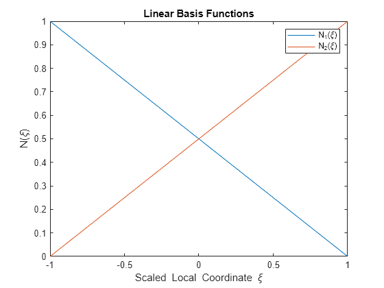
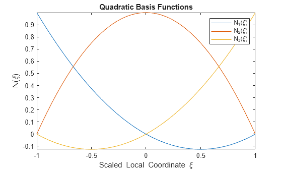
Here, the local coordinate system $$\xi$$ is scaled to range from –1 to 1, the discrete variables $$w_j^i$$, $${\beta }_j^i$$, and $$x_j^i$$ are the nodal values, and $$N_j(\xi )$$ are the shape functions. In this example of FEM analysis, consider two-noded elements ($$m=2$$) and three-noded elements ($$m=3$$) when discretizing each element, where linear and quadratic basis functions are used for these elements, respectively.

To illustrate the linear and quadratic basis functions, define the local coordinate as a symbolic variable xi. Define the linear basis functions and plot them using fplot.

syms xi
N1lin(xi) = (1 - xi)/2;
N2lin(xi) = (1 + xi)/2;
Nlin(xi) = [N1lin; N2lin]

Nlin(xi) = 
$$\left(\begin{array}{c}\frac{1}{2}-\frac{\xi }{2}\\ \frac{\xi }{2}+\frac{1}{2}\end{array}\right)$$

fplot(Nlin,[-1 1])
title("Linear Basis Functions")
xlabel("Scaled Local Coordinate \xi")
ylabel("N(\xi)")
legend("N_1(\xi)","N_2(\xi)")

Next, define the quadratic basis functions and plot them using fplot.

N1quad(xi) = xi*(xi - 1)/2;
N2quad(xi) = -(xi - 1)*(xi + 1);
N3quad(xi) = xi*(xi + 1)/2;
Nquad(xi) = [N1quad; N2quad; N3quad]

Nquad(xi) = 
$$\left(\begin{array}{c}\frac{\xi \hspace{0.17em}\left(\xi -1\right)}{2}\\ -\left(\xi -1\right)\hspace{0.17em}\left(\xi +1\right)\\ \frac{\xi \hspace{0.17em}\left(\xi +1\right)}{2}\end{array}\right)$$

figure
fplot(Nquad,[-1 1])
title("Quadratic Basis Functions")
xlabel("Scaled Local Coordinate \xi")
ylabel("N(\xi)")
legend("N_1(\xi)","N_2(\xi)","N_3(\xi)")

This Timoshenko beam model can suffer from transverse shear locking. In the thin beam limit, the Timoshenko beam model must satisfy the Kirchhoff constraint $$\gamma =0$$ and the constraint $$\kappa =0$$. These constraints yield the trivial solution of the nodal displacements as $$w_j^i={\beta }_j^i=0$$. In other words, the element locks. The lower-order basis functions cause an erroneous stiffening to occur, which restricts the transverse shear deformation and leads to an overestimation of the beam's stiffness. The term locking refers to this artificial stiffening, as if the beam's cross sections are locked together and unable to shear properly relative to each other. To alleviate this problem, you can use higher-order basis functions for smaller errors in the FEM analysis to solve the Timoshenko beam problem.

Generate Two-Noded and Three-Noded Mesh Elements

Define the functions that generate two-noded and three-noded mesh elements. These functions return the meshes as a structure with fields that represent the number of elements, the global node coordinates, the node indices of each element, and the total number of degrees of freedom (DOF).

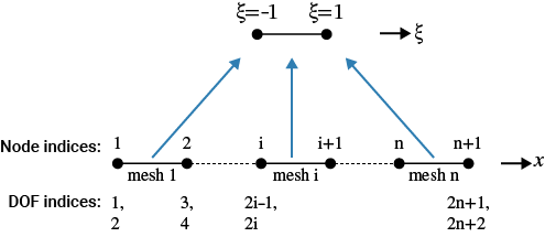
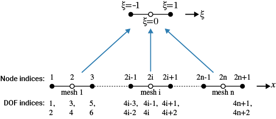
The following figures illustrate the convention used to define the meshes. In this example, the beam is divided into equally spaced elements with the total number of mesh elements defined by n. As a result, the nodal coordinates are equally spaced. The node indices are sequentially numbered from the left end to the right end, starting from 1 up to n+1 for two-noded mesh elements (or 2*n+1 for three-noded mesh elements). Each node has two degrees of freedom, corresponding to the transverse displacement and the bending angle. The indices for these degrees of freedom are labeled 1 and 2 for the first node, respectively, 3 and 4 for the second node, and so on until the final node. Consequently, the total number of degrees of freedom is twice the total number of nodes.

This figure illustrates a linear mesh with two-noded mesh elements, where n is the number of mesh elements. Node indices range from 1 to n+1. DOF indices range from 1 to 2*n+2.

Define a function that generates two-noded mesh elements.

function mshLin = generateLinearMesh(L,n)
mshLin.n = n;
mshLin.nodes = linspace(0,L,n + 1)';
mshLin.elements = (1:n)' + [0 1];
mshLin.numDOFs = 2*length(mshLin.nodes);
end

This figure illustrates a quadratic mesh with three-noded mesh elements, where n is the number of mesh elements. Node indices range from 1 to 2*n+1. DOF indices range from 1 to 4*n+2.

Define a function that generates three-noded mesh elements.

function mshQuad = generateQuadraticMesh(xend,n)
mshQuad.n = n;
mshQuad.nodes = linspace(0,xend,2*n + 1)';
mshQuad.elements = 2*(1:n)' + [-1 0 1];
mshQuad.numDOFs = 2*length(mshQuad.nodes);
end

Using these functions, generate a linear mesh with 30 two-noded mesh elements and a quadratic mesh with 30 three-noded mesh elements.

n = 30;
mshLin = generateLinearMesh(beamParams.L,n)

mshLin = struct with fields:
           n: 30
       nodes: [31x1 double]
    elements: [30x2 double]
     numDOFs: 62

mshQuad = generateQuadraticMesh(beamParams.L,n)

mshQuad = struct with fields:
           n: 30
       nodes: [61x1 double]
    elements: [30x3 double]
     numDOFs: 122

Assemble Global Stiffness Matrix and Load Vector

The FEM discretizes the beam into a finite number of elements and solves for the displacement fields. In this analysis, the global stiffness matrix connects the vector of nodal displacements with the vector of forces. In other words, the FEM solves the matrix equation of the form $\mathbf{F}=\mathbf{K}\mathbf{d}$, where $\mathbf{F}$ is the load vector, $\mathbf{K}$ is the global stiffness matrix, and $\mathbf{d}$ is the nodal displacement vector. This section discusses the steps to derive the global stiffness matrix and how to reformulate the equilibrium equations into the matrix equation of the form $\mathbf{F}=\mathbf{K}\mathbf{d}$.

To derive this matrix equation, first apply the virtual work principle to the Timoshenko beam model. This principle states that the sum of the internal and external virtual work is zero with respect to infinitesimal virtual displacements, which are small variational displacements satisfying the boundary conditions of the system. Multiply the two equilibrium equations (Equations 1–2) by arbitrary variations $\delta \mathit{w}$ and $\delta \beta$, respectively. Then, perform integration by parts and apply the corresponding Dirichlet and Neumann boundary conditions.

$$\begin{array}{l}{\int }_0^{\mathit{L}}\left(\frac{\mathit{dQ}}{\mathit{dx}}+\mathit{q}\right)\delta \mathit{w}\mathit{dx}=0\Rightarrow \\ -{\int }_0^{\mathit{L}}\mathit{Q}\delta \frac{\mathit{dw}}{\mathit{dx}}\mathit{dx}+\mathit{Q}\left(\mathit{L}\right)\delta \mathit{w}\left(\mathit{L}\right)-\mathit{Q}\left(0\right)\delta \mathit{w}\left(0\right)+{\int }_0^{\mathit{L}}\mathit{q}\delta \mathit{w}\mathit{dx}=0,\\ {\int }_0^{\mathit{L}}\left(\frac{\mathit{dM}}{\mathit{dx}}-\mathit{Q}+\mathit{m}\right)\delta \beta \mathit{dx}=0\Rightarrow \\ -{\int }_0^{\mathit{L}}\mathit{M}\delta \frac{\mathit{d}\beta }{\mathit{dx}}\mathit{dx}-{\int }_0^{\mathit{L}}\mathit{Q}\delta \beta \mathit{dx}+\mathit{M}\left(\mathit{L}\right)\delta \beta \left(\mathit{L}\right)-\mathit{M}\left(0\right)\delta \beta \left(0\right)+{\int }_0^{\mathit{L}}\mathit{m}\delta \beta \mathit{dx}=0.\end{array}$$

Add the two equations to obtain the final form of the total weak formulation of the Timoshenko beam problem.

$$\begin{array}{l}\stackrel{\delta W_{\text{int}}}{\overbrace{\underset{}{-{\int }_0^{L}Q(\frac{d\delta w}{dx}+\delta \beta )dx-{\int }_0^{L}M\frac{d\delta \beta }{dx}dx}}}+\stackrel{\delta W_{\text{ext}}}{\overbrace{\underset{}{{\int }_0^{L}q\delta wdx+{\int }_0^{L}m\delta \beta dx}}}\\ +\stackrel{\text{boundary}\text{terms}}{\overbrace{\underset{}{Q(0)\delta w(0)+Q(L)\delta w(L)+M(0)\delta \beta (0)+M(L)\delta \beta (L)}}}=0.\end{array}$$

Next, cast this formulation into matrix form by defining these vectors and matrices.

• $\mathbf{u}=\left[\begin{array}{c}\mathit{w}\\ \beta \end{array}\right]$ is the displacements.

• $\epsilon =\left[\begin{array}{c}\gamma \\ \kappa \end{array}\right]=\mathbf{L}\cdot \mathbf{u}$ is the strains, where $\mathbf{L}=\left[\begin{array}{cc}\frac{\partial }{\partial \mathit{x}}& 1\\ 0& \frac{\partial }{\partial \mathit{x}}\end{array}\right]$.

• $\sigma =\left[\begin{array}{c}\mathit{Q}\\ \mathit{M}\end{array}\right]=\mathbf{C}\cdot \epsilon$ is the internal loads, where $\mathbf{C}=\left[\begin{array}{cc}\alpha \mathit{GA}& 0\\ 0& \mathit{EI}\end{array}\right]$.

• $\mathbf{p}=\left[\begin{array}{c}\mathit{q}\\ \mathit{m}\end{array}\right]$ is the external loads.

• ${\mathbf{P}}_0=\left[\begin{array}{c}\mathit{Q}\left(0\right)\\ \mathit{M}\left(0\right)\end{array}\right]$ and ${\mathbf{P}}_{\mathit{L}}=\left[\begin{array}{c}\mathit{Q}\left(\mathit{L}\right)\\ \mathit{M}\left(\mathit{L}\right)\end{array}\right]$ are forces on the boundaries.

The matrix formulation of the Timoshenko beam problem becomes:

$${\int }_0^{\mathit{L}}\left({\sigma }^{\mathit{T}}\cdot \delta \epsilon -{\mathbf{p}}^{\mathit{T}}\cdot \delta \mathbf{u}\right)\mathit{dx}-{\mathit{P}}_0^{\mathit{T}}\cdot \delta \mathbf{u}\left(0\right)-{\mathit{P}}_{\mathit{L}}^{\mathit{T}}\cdot \delta \mathbf{u}\left(\mathit{L}\right)=0.$$

Next, discretize the beam model by specifying the elements and selecting the appropriate basis functions for the given number of nodes within each mesh element. Here, $$x_1^i$$ and $$x_m^i$$ are the global coordinates of the end locations of the element with index $$i$$. For an element with $$m$$ nodes, the approximated displacements of each element in terms of the nodal displacements are

$${\mathbf{u}}^{\mathit{i}}=\mathbf{N}\cdot {\mathbf{d}}^{\mathit{i}},$$

where

$$\begin{array}{l}\mathbf{N}=\left[\begin{array}{ccccc}{\mathit{N}}_1& 0& ...& {\mathit{N}}_{\mathit{m}}& 0\\ 0& {\mathit{N}}_1& ...& 0& {\mathit{N}}_{\mathit{m}}\end{array}\right],\\ {\mathbf{d}}^{\mathit{i}}=\left[\begin{array}{c}{{\mathit{w}}^{\mathit{i}}}_1\\ {{\beta }^{\mathit{i}}}_1\\ ⋮\\ {{\mathit{w}}^{\mathit{i}}}_{\mathit{m}}\\ {{\beta }^{\mathit{i}}}_{\mathit{m}}\end{array}\right].\end{array}$$

The approximated strains of each element are

$${\epsilon }^{\mathit{i}}=\mathbf{L}\cdot {\mathbf{u}}^{\mathit{i}}=\mathbf{B}\cdot {\mathbf{d}}^{\mathit{i}},$$

where

$\mathbf{B}=\mathbf{L}\mathbf{N}=\left[\begin{array}{ccccc}\frac{\partial {\mathit{N}}_1}{\partial \mathit{x}}& {\mathit{N}}_1& ...& \frac{\partial {\mathit{N}}_{\mathit{m}}}{\partial \mathit{x}}& {\mathit{N}}_{\mathit{m}}\\ 0& \frac{\partial {\mathit{N}}_1}{\partial \mathit{x}}& ...& 0& \frac{\partial {\mathit{N}}_{\mathit{m}}}{\partial \mathit{x}}\end{array}\right]$.

The formulation of the virtual work principle for each element, which must hold for any virtual displacements $\delta {\mathbf{d}}^{\mathit{i}}$, becomes:

$${\int }_{{\mathit{x}}_1^{\mathit{i}}}^{{\mathit{x}}_{\mathit{m}}^{\mathit{i}}}\left({{\mathbf{d}}^{\mathit{i}}}^{\mathit{T}}{\mathbf{B}}^{\mathit{T}}{\mathbf{C}}^{\mathit{T}}\mathbf{B}\cdot \delta {\mathbf{d}}^{\mathit{i}}-{\mathbf{p}}^{\mathit{T}}\mathbf{N}\cdot \delta {\mathbf{d}}^{\mathit{i}}\right)\mathit{dx}-{\left[\begin{array}{c}{\mathbf{P}}_{{\mathit{x}}_1^{\mathit{i}}}\\ {\mathbf{P}}_{{\mathit{x}}_{\mathit{m}}^{\mathit{i}}}\end{array}\right]}^{\mathit{T}}\cdot \delta {\mathbf{d}}^{\mathit{i}}=0.$$

(3)

For elements $$i$$ and $$i+1$$ that are connected to each other, the nodal displacements and the global coordinates of the right end of element $$i$$ and the left end of the adjacent element $$i+1$$ are related to each other. For the basis functions in this example, the nodal displacements and global coordinates are continuous between the adjacent elements. In other words, this formulation yields the relations $$w_m^i=w_1^{i+1}$$, $${\beta }_m^i={\beta }_1^{i+1}$$, and $$x_m^i=x_1^{i+1}$$.

Next, rewrite the virtual work formulation in Equation 3 by transposing the matrix multiplications, which results in the local stiffness matrix representation of each element.

$$\begin{array}{l}{\int }_{{\mathit{x}}_1^{\mathit{i}}}^{{\mathit{x}}_{\mathit{m}}^{\mathit{i}}}\left({\mathbf{B}}^{\mathit{T}}\mathbf{C}\mathbf{B}\mathrm{dx}\right){\mathbf{d}}^{\mathit{i}}-{\int }_{{\mathit{x}}_1^{\mathit{i}}}^{{\mathit{x}}_{\mathit{m}}^{\mathit{i}}}{\mathbf{N}}^{\mathit{T}}\mathbf{p}\mathit{dx}-\left[\begin{array}{c}{\mathbf{P}}_{{\mathit{x}}_1^{\mathit{i}}}\\ {\mathbf{P}}_{{\mathit{x}}_{\mathit{m}}^{\mathit{i}}}\end{array}\right]=0,\\ {\mathbf{K}}^{\mathit{i}}\cdot {\mathbf{d}}^{\mathit{i}}={\mathbf{F}}^{\mathit{i}}.\end{array}$$

Here, the local stiffness matrix is ${\mathbf{K}}^{\mathit{i}}={\int }_{{\mathit{x}}_1^{\mathit{i}}}^{{\mathit{x}}_{\mathit{m}}^{\mathit{i}}}{\mathbf{B}}^{\mathit{T}}\mathbf{C}\mathbf{B}\mathrm{dx}$ and the local load vector is ${\mathbf{F}}^{\mathit{i}}={\int }_{{\mathit{x}}_1^{\mathit{i}}}^{{\mathit{x}}_{\mathit{m}}^{\mathit{i}}}{\mathbf{N}}^{\mathit{T}}\mathbf{p}\mathit{dx}-\left[\begin{array}{c}{\mathbf{P}}_{{\mathit{x}}_1^{\mathit{i}}}\\ {\mathbf{P}}_{{\mathit{x}}_{\mathit{m}}^{\mathit{i}}}\end{array}\right]$.

Next, assemble the global stiffness matrix $\mathbf{K}$ and load vector $\mathbf{F}$ by following these steps:

1. Initialize a global stiffness matrix and a global load vector, both filled with zeros. The dimensions of the matrix and vector depend on the total number of nodes in the system and the degrees of freedom per node.

2. Compute the local stiffness matrix and load vector of each mesh element. Because the basis functions are defined in terms of the local coordinates $$\xi$$ rather than the global coordinates $$x$$, you must apply the required transformations when performing the integration that involves these basis functions and their derivatives.

3. Determine the global node indices associated with the local nodes of the element. For each degree of freedom in the element, add the element's local stiffness matrix values to the corresponding positions in the global stiffness matrix. These positions are determined by the global node indices.

4. Similarly, add the element's local load vector values to the corresponding positions in the global load vector. In this step, you do not need to account for the $\left[\begin{array}{c}{\mathbf{P}}_{{\mathit{x}}_1^{\mathit{i}}}\\ {\mathbf{P}}_{{\mathit{x}}_{\mathit{m}}^{\mathit{i}}}\end{array}\right]$ terms in the local load vectors. According to Newton's third law, which states that for every action, there is an equal and opposite reaction, the boundary forces between connected elements $$i$$ and $$i+1$$ cancel each other out, or ${\mathbf{P}}_{{\mathit{x}}_{\mathit{m}}^{\mathit{i}}}={-\mathbf{P}}_{{\mathit{x}}_1^{\mathit{i}+1}}$.

5. Loop over all elements and add their contributions to the global stiffness matrix and load vector by combining the local stiffness matrices and load vectors into a single global stiffness matrix and load vector.

Because this example describes a 1-D beam model, the transformation from local coordinates to the global coordinate involves only the derivative function $\partial \mathit{x}/\partial \xi$ and its inverse. For a model with a higher dimension, such as the 2-D Reissner–Mindlin plate, the coordinate transformation might involve the Jacobian matrix of the global coordinate vector and its determinant.

Define the assembleGlobalKF function to construct the global stiffness matrix and load vector. The inputs to this function are the mesh structure, basis functions, and beam parameters. In this example, consider the external loads as constants, where $$q(x)=\underset{}{\overset{‾}{q}}$$ and $$m(x)=\underset{}{\overset{‾}{m}}$$.

function [K,F] = assembleGlobalKF(msh,N_basis,beamParams)

xi = sym("xi");
nNodesPerElement = length(N_basis(xi));
nDOFsPerElement = 2*nNodesPerElement;

x_basis = sym("x_basis",[nNodesPerElement 1]);
x = N_basis'*x_basis;
dN(xi) = diff(N_basis,xi)*inv(diff(x,xi));

alpha = sym("alpha");
G = sym("G");
A = sym("A");
E = sym("E");
I = sym("I");
q_bar = sym("q_bar");
m_bar = sym("m_bar");

C = [alpha*G*A  0;
     0          E*I];

Nmtx = sym(zeros(2,nDOFsPerElement));
Bmtx = sym(zeros(2,nDOFsPerElement));
Nformula = formula(N_basis);
dNformula = formula(dN);

for ii = 1:nNodesPerElement
    Nmtx(1, 2*ii - 1) = Nformula(ii);
    Nmtx(2, 2*ii) = Nformula(ii);
    Bmtx(1, 2*ii - 1) = dNformula(ii);
    Bmtx(1, 2*ii) = Nformula(ii);
    Bmtx(2, 2*ii) = dNformula(ii);
end

K = zeros(msh.numDOFs);
F = zeros(msh.numDOFs,1);

for ii = 1:msh.n
    id = msh.elements(ii,:);
    coords = msh.nodes(id);
    
    KEintegrand = Bmtx.'*C*Bmtx*diff(x,xi);
    KEintegrand = subs(KEintegrand,beamParams);
    KEintegrand = subs(KEintegrand,x_basis,coords);

    FEintegrand = Nmtx.'*[q_bar; m_bar]*diff(x,xi);
    FEintegrand = subs(FEintegrand,beamParams);
    FEintegrand = subs(FEintegrand,x_basis,coords);

    KE = int(KEintegrand,xi,-1,1);
    FE = int(FEintegrand,xi,-1,1);

    idFill = vertcat(2*id - 1, 2*id);
    idFill = idFill(:);
    K(idFill,idFill) = K(idFill,idFill) + KE;
    F(idFill) = F(idFill) + FE;
end

end

After assembling the global stiffness matrix and load vector, you can apply the necessary boundary conditions for the fixed displacements. This application typically involves modifying rows and columns of the global stiffness matrix and adjusting the global load vector accordingly. Finally, you can solve the global system of equations in the form of $\mathbf{F}=\mathbf{K}\mathbf{d}$ for $\mathbf{d}$, which represents the unknown nodal displacements. From these displacements, you can compute other quantities of interest, such as the strains and stresses in the mesh elements.

Find FEM Solution Using Linear Basis for Two-Noded Elements

Find the FEM solution for the cantilever beam by using the approximation of a linear basis with two-noded mesh elements. Construct the global stiffness matrix and load vector using the assembleGlobalKF function.

[K,F] = assembleGlobalKF(mshLin,Nlin,beamParams);

Define the fixed degrees of freedom for the cantilever beam. The indices for these degrees of freedom are 1 and 2, corresponding to the fixed leftmost node, without any transverse displacement and bending rotation. Define the free degrees of freedom of the mesh elements by excluding the fixed degrees of freedom.

fixedDOFs = 1:2;
freeDOFs = 1:mshLin.numDOFs;
freeDOFs = setdiff(freeDOFs,fixedDOFs);

Compute the nodal displacements of the cantilever beam from the global stiffness matrix and load vector.

u = zeros(mshLin.numDOFs,1);
u(freeDOFs) = K(freeDOFs,freeDOFs)\F(freeDOFs);

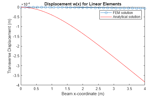
Plot the FEM solution of the transverse displacement $$w(x)$$ of the beam. Compare this plot to the analytical solution. Due to the transverse shear locking effect in a thin beam, where the beam thickness in this example is 0.01 m and the beam length is 4 m, the FEM analysis yields the trivial solution of $\mathit{w}\left(\mathit{x}\right)\approx 0$. For comparison, the next section discusses the analysis using a quadratic basis with three-noded mesh elements, which do not suffer from the transverse shear locking effect.

figure
plot(mshLin.nodes,u(1:2:end,1),"-o")
hold on
fplot(w_eval,[0 beamParams.L],"r-")
hold off
title("Displacement w(x) for Linear Elements")
xlabel("Beam x-coordinate (m)")
ylabel("Transverse Displacement (m)")
legend("FEM solution","Analytical solution")

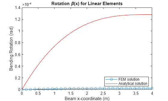
Plot the FEM solution of the bending rotation angle $$\beta (x)$$ of the beam. Due to transverse shear locking, you also obtain the trivial solution $$\beta (x)\approx 0$$ from the FEM analysis, which does not match the analytical solution.

figure
plot(mshLin.nodes,u(2:2:end,1),"-o")
hold on
fplot(beta_eval,[0 beamParams.L],"r-")
hold off
title("Rotation \beta(x) for Linear Elements")
xlabel("Beam x-coordinate (m)")
ylabel("Bending Rotation (rad)")
legend("FEM solution","Analytical solution",Location="southeast")

Find FEM Solution Using Quadratic Basis for Three-Noded Elements

Find the FEM solution for the cantilever beam by using the approximation of a quadratic basis with three-noded mesh elements. Construct the global stiffness matrix and load vector using the assembleGlobalKF function.

[K,F] = assembleGlobalKF(mshQuad,Nquad,beamParams);

Define the fixed degrees of freedom for the cantilever beam. Define the free degrees of freedom of the mesh elements by excluding the fixed degrees of freedom.

fixedDOFs = 1:2;
freeDOFs = 1:mshQuad.numDOFs;
freeDOFs = setdiff(freeDOFs,fixedDOFs);

Compute the nodal displacements of the cantilever beam from the global stiffness matrix and load vector.

u = zeros(mshQuad.numDOFs,1);
u(freeDOFs) = K(freeDOFs,freeDOFs)\F(freeDOFs);

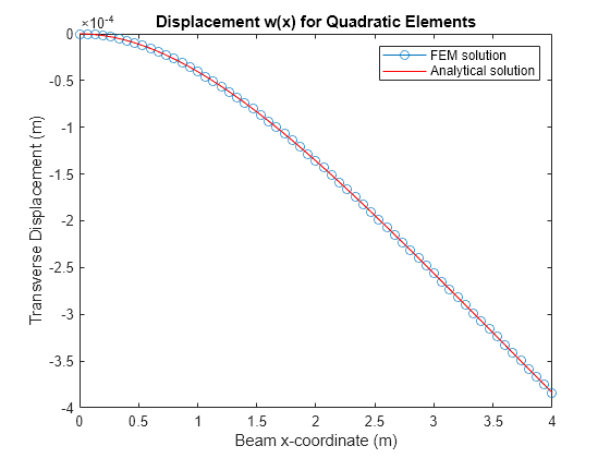
Plot the FEM solution of the transverse displacement $$w(x)$$ of the beam. Compare this plot to the analytical solution. Here, the use of higher-order polynomials in the basis functions reduces the transverse shear locking effect.. The FEM solution matches the analytical solution.

figure
plot(mshQuad.nodes,u(1:2:end,1),"-o")
hold on
fplot(w_eval,[0 beamParams.L],"r-")
hold off
title("Displacement w(x) for Quadratic Elements")
xlabel("Beam x-coordinate (m)")
ylabel("Transverse Displacement (m)")
legend("FEM solution","Analytical solution")

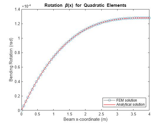
Plot the FEM solution of the bending rotation angle $$\beta (x)$$ of the beam, which matches the analytical solution.

figure
plot(mshQuad.nodes,u(2:2:end,1),"-o")
hold on
fplot(beta_eval,[0 beamParams.L],"r-")
hold off
title("Rotation \beta(x) for Quadratic Elements")
xlabel("Beam x-coordinate (m)")
ylabel("Bending Rotation (rad)")
legend("FEM solution","Analytical solution",Location="southeast")

Find Analytical and FEM Solutions for Beam Fixed at Both Ends

Previous sections discussed the analytical and FEM solutions of a cantilever beam that is fixed at one end and free at the other. This section focuses on a beam that is fixed at both ends. This section applies the previously discussed steps to find the analytical and FEM solutions of the beam displacement.

For a beam that is fixed at both ends, the boundary conditions are $$w(0)=0$$, $$\beta (0)=0$$, $$w(L)=0$$, and $$\beta (L)=0$$.

cond = [w(0)==0; beta(0)==0; w(L)==0; beta(L)==0];

Find the analytical solutions for the beam displacements by using dsolve on the equilibrium equations and the specified boundary conditions.

[beta_sol,w_sol] = dsolve(eqns,cond);
w_sol = simplify(w_sol)

w_sol = 
$$\frac{\bar{q}\hspace{0.17em}x\hspace{0.17em}\left(L-x\right)\hspace{0.17em}\left(-A\hspace{0.17em}G\hspace{0.17em}\alpha \hspace{0.17em}{x}^2+A\hspace{0.17em}G\hspace{0.17em}L\hspace{0.17em}\alpha \hspace{0.17em}x+12\hspace{0.17em}\text{E}\hspace{0.17em}\text{I}\right)}{24\hspace{0.17em}A\hspace{0.17em}\text{E}\hspace{0.17em}G\hspace{0.17em}\text{I}\hspace{0.17em}\alpha }$$

beta_sol = simplify(beta_sol)

beta_sol = 
$$-\frac{\bar{q}\hspace{0.17em}x\hspace{0.17em}\left(L^2-3\hspace{0.17em}L\hspace{0.17em}x+2\hspace{0.17em}{x}^2\right)}{12\hspace{0.17em}\text{E}\hspace{0.17em}\text{I}}$$

Next, evaluate these solutions for the known values of the beam parameters.

w_eval = subs(w_sol,beamParams);
beta_eval = subs(beta_sol,beamParams);

To obtain the FEM solutions, construct the global stiffness matrix and load vector for the two-noded mesh elements with linear basis functions using the previously generated linear meshs.

[K,F] = assembleGlobalKF(mshLin,Nlin,beamParams);

Define the fixed degrees of freedom for the beam that is fixed at both ends according to the boundary conditions. The indices for these degrees of freedom are 1 and 2, corresponding to the fixed leftmost node, and numDOFs - 1 and numDOFs, corresponding to the fixed rightmost end, where numDOFs is the total number of degrees of freedom. Define the free degrees of freedom of the mesh elements by excluding the fixed degrees of freedom.

fixedDOFs = [1:2 mshLin.numDOFs-1:mshLin.numDOFs];
freeDOFs = 1:mshLin.numDOFs;
freeDOFs = setdiff(freeDOFs,fixedDOFs);

Compute the nodal displacements of the beam that is fixed at both ends from the global stiffness matrix and load vector.

u = zeros(mshLin.numDOFs,1);
u(freeDOFs) = K(freeDOFs,freeDOFs)\F(freeDOFs);

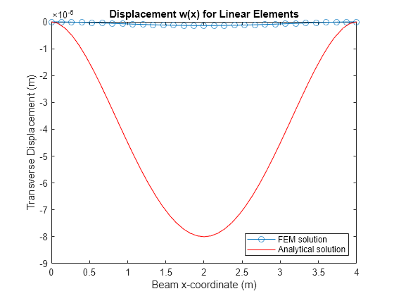
Plot the analytical and FEM solutions of the transverse displacement $$w(x)$$ of the beam. Due to the transverse shear locking effect in a thin beam, the FEM analysis using linear basis functions yields the trivial solution $\mathit{w}\left(\mathit{x}\right)\approx 0$, which does not match the analytical solution.

figure
plot(mshLin.nodes,u(1:2:end,1),"-o")
hold on
fplot(w_eval,[0 beamParams.L],"r-")
hold off
title("Displacement w(x) for Linear Elements")
xlabel("Beam x-coordinate (m)")
ylabel("Transverse Displacement (m)")
legend("FEM solution","Analytical solution",Location="southeast")

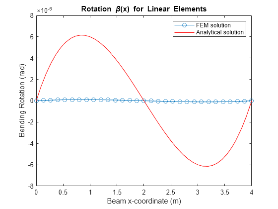
Plot the analytical and FEM solutions of the bending rotation angle $$\beta (x)$$ of the beam. The FEM solution of the bending rotation angle is also the trivial solution $$\beta (x)\approx 0$$, which does not match the analytical solution.

figure
plot(mshLin.nodes,u(2:2:end,1),"-o")
hold on
fplot(beta_eval,[0 beamParams.L],"r-")
hold off
title("Rotation \beta(x) for Linear Elements")
xlabel("Beam x-coordinate (m)")
ylabel("Bending Rotation (rad)")
legend("FEM solution","Analytical solution")

To obtain better FEM solutions, construct the global stiffness matrix and load vector for the three-noded mesh elements with quadratic basis functions using the previously generated quadratic mesh.

[K,F] = assembleGlobalKF(mshQuad,Nquad,beamParams);

Define the fixed degrees of freedom for the beam that is fixed at both ends according to the boundary conditions. Define the free degrees of freedom of the mesh elements by excluding the fixed degrees of freedom.

fixedDOFs = [1:2 mshQuad.numDOFs-1:mshQuad.numDOFs];
freeDOFs = 1:mshQuad.numDOFs;
freeDOFs = setdiff(freeDOFs,fixedDOFs);

Compute the nodal displacements of the beam from the global stiffness matrix and load vector.

u = zeros(mshQuad.numDOFs,1);
u(freeDOFs) = K(freeDOFs,freeDOFs)\F(freeDOFs);

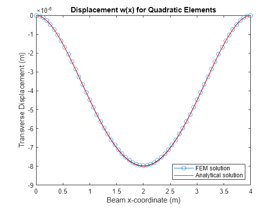
Plot the analytical and FEM solutions of the transverse displacement $$w(x)$$ of the beam. The use of higher-order polynomials in the basis functions reduces the transverse shear locking effect, and the FEM solution matches the analytical solution.

figure
plot(mshQuad.nodes,u(1:2:end,1),"-o")
hold on
fplot(w_eval,[0 beamParams.L],"r-")
hold off
title("Displacement w(x) for Quadratic Elements")
xlabel("Beam x-coordinate (m)")
ylabel("Transverse Displacement (m)")
legend("FEM solution","Analytical solution",Location="southeast")

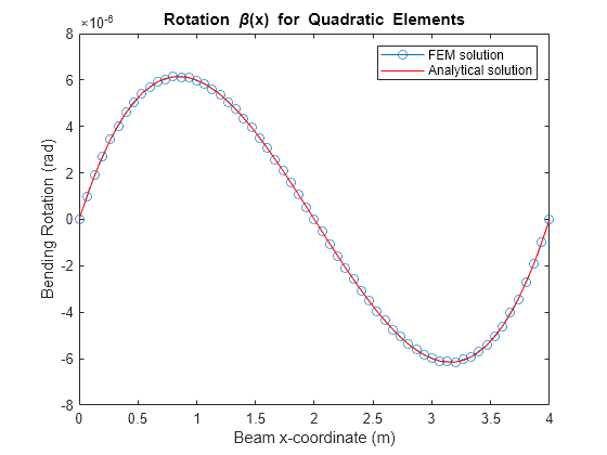
Plot the FEM solution of the bending rotation angle $$\beta (x)$$ of the beam, which also matches the analytical solution.

figure
plot(mshQuad.nodes,u(2:2:end,1),"-o")
hold on
fplot(beta_eval,[0 beamParams.L],"r-")
hold off
title("Rotation \beta(x) for Quadratic Elements")
xlabel("Beam x-coordinate (m)")
ylabel("Bending Rotation (rad)")
legend("FEM solution","Analytical solution")

References

[1] Öchsner, Andreas. Classical Beam Theories of Structural Mechanics. Cham: Springer International Publishing, 2021. https://doi.org/10.1007/978-3-030-76035-9.

[2] Hughes, Thomas JR. The Finite Element Method: Linear Static and Dynamic Finite Element Analysis. Dover Publications, 1st edition, 2000.

[3] Bittencourt, Marco L. Computational Solid Mechanics: Variational Formulation and High Order Approximation. Boca Raton, FL: CRC Press, 2014. https://doi.org/10.1201/b16392.

[4] Reddy, J N. “On the Dynamic Behaviour of the Timoshenko Beam Finite Elements.” Sadhana 24, no. 3 (June 1999): 175–98. https://doi.org/10.1007/BF02745800.