Main Content

factoran

Factor analysis

Description

factoran computes the maximum likelihood estimate (MLE) of the factor loadings matrix Λ in the factor analysis model

x=μ+Λf+e

where x is a vector of observed variables, μ is a constant vector of means, Λ is a constant d-by-m matrix of factor loadings, f is a vector of independent, standardized common factors, and e is a vector of independent specific factors. x, μ, and e each has length d. f has length m.

Alternatively, the factor analysis model can be specified as

cov(x)=ΛΛT+Ψ

where Ψ=cov(e) is a d-by-d diagonal matrix of specific variances.

For the uses of factoran and its relation to pca, see Perform Factor Analysis on Exam Grades.

example

lambda = factoran(X,m) returns the factor loadings matrix lambda for the data matrix X with m common factors.

example

[lambda,psi] = factoran(X,m) also returns maximum likelihood estimates of the specific variances.

example

[lambda,psi,T] = factoran(X,m) also returns the m-by-m factor loadings rotation matrix T.

example

[lambda,psi,T,stats] = factoran(X,m) also returns the structure stats containing information relating to the null hypothesis H0 that the number of common factors is m.

example

[lambda,psi,T,stats,F] = factoran(X,m) also returns predictions of the common factors (factor scores).

example

___ = factoran(X,m,Name,Value) modifies the model fit and outputs using one or more name-value pair arguments, for any output arguments in the previous syntaxes. For example, you can specify that the X data is a covariance matrix.

Examples

collapse all

Create some pseudorandom raw data.

rng default % For reproducibility
n = 100;
X1 = 5 + 3*rand(n,1); % Factor 1
X2 = 20 - 5*rand(n,1); % Factor 2

Create six data vectors from the raw data, and add random noise.

Y1 = 2*X1 + 3*X2 + randn(n,1);
Y2 = 4*X1 + X2 + 2*randn(n,1);
Y3 = X1 - X2 + 3*randn(n,1);
Y4 = -2*X1 + 4*X2 + 4*randn(n,1);
Y5 = 3*(X1 + X2) + 5*randn(n,1);
Y6 = X1 - X2/2 + 6*randn(n,1);

Create a data matrix from the data vectors.

X = [Y1,Y2,Y3,Y4,Y5,Y6];

Extract the two factors from the noisy data matrix X using factoran. Display the outputs.

m = 2;
[lambda,psi,T,stats,F] = factoran(X,m);
disp(lambda)
    0.8666    0.4828
    0.8688   -0.0998
   -0.0131   -0.5412
    0.2150    0.8458
    0.7040    0.2678
   -0.0806   -0.2883
disp(psi)
    0.0159
    0.2352
    0.7070
    0.2385
    0.4327
    0.9104
disp(T)
    0.8728    0.4880
    0.4880   -0.8728
disp(stats)
    loglike: -0.0531
        dfe: 4
      chisq: 5.0335
          p: 0.2839
disp(F(1:10,:))
    1.8845   -0.6568
   -0.1714   -0.8113
   -1.0534    2.0743
    1.0390   -1.1784
    0.4309    0.9907
   -1.1823    0.6570
   -0.2129    1.1898
   -0.0844   -0.7421
    0.5854   -1.1379
    0.8279   -1.9624

View the correlation matrix of the data.

corrX = corr(X)
corrX = 6×6

    1.0000    0.7047   -0.2710    0.5947    0.7391   -0.2126
    0.7047    1.0000    0.0203    0.1032    0.5876    0.0289
   -0.2710    0.0203    1.0000   -0.4793   -0.1495    0.1450
    0.5947    0.1032   -0.4793    1.0000    0.3752   -0.2134
    0.7391    0.5876   -0.1495    0.3752    1.0000   -0.2030
   -0.2126    0.0289    0.1450   -0.2134   -0.2030    1.0000

Compare corrX to its corresponding values returned by factoran, lambda*lambda' + diag(psi).

C0 = lambda*lambda' + diag(psi)
C0 = 6×6

    1.0000    0.7047   -0.2726    0.5946    0.7394   -0.2091
    0.7047    1.0000    0.0426    0.1023    0.5849   -0.0413
   -0.2726    0.0426    1.0000   -0.4605   -0.1542    0.1571
    0.5946    0.1023   -0.4605    1.0000    0.3779   -0.2611
    0.7394    0.5849   -0.1542    0.3779    1.0000   -0.1340
   -0.2091   -0.0413    0.1571   -0.2611   -0.1340    1.0000

factoran obtains lambda and psi that correspond closely to the correlation matrix of the original data.

View the results without using rotation.

[lambda,psi,T,stats,F] = factoran(X,m,'Rotate','none');
disp(lambda)
    0.9920    0.0015
    0.7096    0.5111
   -0.2755    0.4659
    0.6004   -0.6333
    0.7452    0.1098
   -0.2111    0.2123
disp(psi)
    0.0159
    0.2352
    0.7070
    0.2385
    0.4327
    0.9104
disp(T)
     1     0
     0     1
disp(stats)
    loglike: -0.0531
        dfe: 4
      chisq: 5.0335
          p: 0.2839
disp(F(1:10,:))
    1.3243    1.4929
   -0.5456    0.6245
    0.0928   -2.3246
    0.3318    1.5356
    0.8596   -0.6544
   -0.7114   -1.1504
    0.3947   -1.1424
   -0.4358    0.6065
   -0.0444    1.2789
   -0.2350    2.1169

Compute the factors using only the covariance matrix of X.

X2 = cov(X);
[lambda2,psi2,T2,stats2] = factoran(X2,m,'Xtype','covariance','Nobs',n)
lambda2 = 6×2

    0.8666    0.4828
    0.8688   -0.0998
   -0.0131   -0.5412
    0.2150    0.8458
    0.7040    0.2678
   -0.0806   -0.2883

psi2 = 6×1

    0.0159
    0.2352
    0.7070
    0.2385
    0.4327
    0.9104

T2 = 2×2

    0.8728    0.4880
    0.4880   -0.8728

stats2 = struct with fields:
    loglike: -0.0531
        dfe: 4
      chisq: 5.0335
          p: 0.2839

The results are the same as with the raw data, except factoran cannot compute the factor scores matrix F for covariance data.

Load the sample data.

load carbig

Define the variable matrix.

X = [Acceleration Displacement Horsepower MPG Weight]; 
X = X(all(~isnan(X),2),:);

Estimate the factor loadings using a minimum mean squared error prediction for a factor analysis with two common factors.

[Lambda,Psi,T,stats,F] = factoran(X,2,'Scores','regression');
inv(T'*T);   % Estimated correlation matrix of F, == eye(2)
Lambda*Lambda' + diag(Psi); % Estimated correlation matrix
Lambda*inv(T);              % Unrotate the loadings
F*T';                       % Unrotate the factor scores

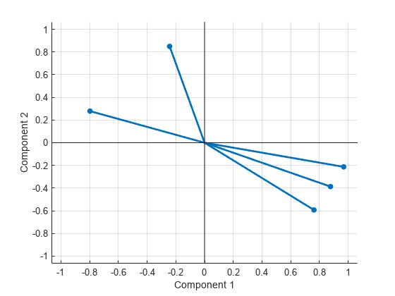
Create a biplot of two factors.

biplot(Lambda,'LineWidth',2,'MarkerSize',20)

Estimate the factor loadings using the covariance (or correlation) matrix.

[Lambda,Psi,T] = factoran(cov(X),2,'Xtype','covariance')
Lambda = 5×2

   -0.2432   -0.8500
    0.8773    0.3871
    0.7618    0.5930
   -0.7978   -0.2786
    0.9692    0.2129

Psi = 5×1

    0.2184
    0.0804
    0.0680
    0.2859
    0.0152

T = 2×2

    0.9476    0.3195
    0.3195   -0.9476

(You could instead use corrcoef(X) instead of cov(X) to create the data for factoran.) Although the estimates are the same, the use of a covariance matrix rather than raw data prevents you from requesting the scores or significance level.

Use promax rotation.

[Lambda,Psi,T,stats,F] = factoran(X,2,'Rotate','promax','power',4);
inv(T'*T)                            % Estimated correlation of F, no longer eye(2)
ans = 2×2

    1.0000   -0.6391
   -0.6391    1.0000

Lambda*inv(T'*T)*Lambda'+diag(Psi)   % Estimated correlation of X
ans = 5×5

    1.0000   -0.5424   -0.6893    0.4309   -0.4167
   -0.5424    1.0000    0.8979   -0.8078    0.9328
   -0.6893    0.8979    1.0000   -0.7730    0.8647
    0.4309   -0.8078   -0.7730    1.0000   -0.8326
   -0.4167    0.9328    0.8647   -0.8326    1.0000

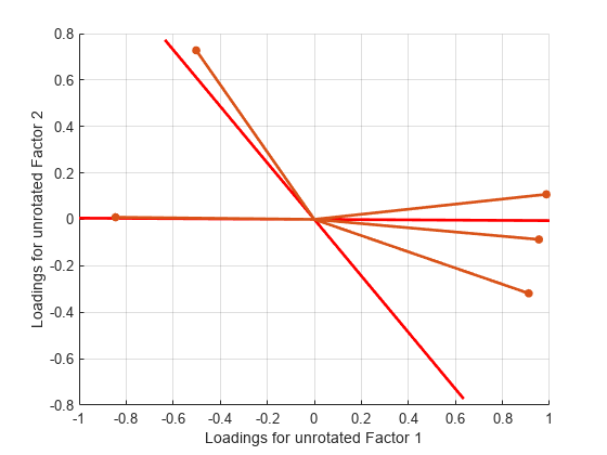
Plot the unrotated variables with oblique axes superimposed.

invT = inv(T);
Lambda0 = Lambda*invT;
figure()
line([-invT(1,1) invT(1,1) NaN -invT(2,1) invT(2,1)], ...
     [-invT(1,2) invT(1,2) NaN -invT(2,2) invT(2,2)], ...
     'Color','r','LineWidth',2)
grid on
hold on
biplot(Lambda0,'LineWidth',2,'MarkerSize',20)       
xlabel('Loadings for unrotated Factor 1')
ylabel('Loadings for unrotated Factor 2')

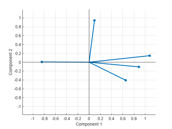
Plot the rotated variables against the oblique axes.

figure()
biplot(Lambda,'LineWidth',2,'MarkerSize',20)

Input Arguments

collapse all

Data, specified as an n-by-d matrix, where each row is an observation of d variables.

Data Types: double

Number of common factors, specified as a positive integer.

Example: 3

Data Types: double

Name-Value Arguments

Specify optional pairs of arguments as Name1=Value1,...,NameN=ValueN, where Name is the argument name and Value is the corresponding value. Name-value arguments must appear after other arguments, but the order of the pairs does not matter.

Before R2021a, use commas to separate each name and value, and enclose Name in quotes.

Example: lambda = factoran(X,m,'Start',10,'Scores','Thomson') specifies to use a starting point for specific variances of 10 and the Thomson method for predicting factor scores.

Input data type of X, specified as the comma-separated pair consisting of 'Xtype' and one of the following:

  • 'data'X is raw data.

  • 'covariance'X is a positive definite covariance or correlation matrix.

Example: 'Xtype','covariance'

Data Types: char | string

Method for predicting factor scores, specified as the comma-separated pair consisting of 'Scores' and one of the following:

  • 'wls' or the equivalent 'Bartlett' — Weighted least-squares estimate treating F as fixed

  • 'regression' or the equivalent 'Thomson' — Minimum mean squared error prediction that is equivalent to a ridge regression

Example: 'Scores','regression'

Data Types: char | string

Starting point for the specific variances psi in the maximum likelihood optimization, specified as the comma-separated pair consisting of 'Start' and one of the following:

  • 'Rsquared' — Chooses the starting vector as a scale factor times diag(inv(corrcoef(X))) (default). For examples, see Jöreskog [2].

  • 'random' — Chooses d uniformly distributed values on the interval [0,1].

  • Positive integer — Performs the given number of maximum likelihood fits, each initialized in the same way as 'random'. factoran returns the fit with the highest likelihood.

  • Matrix with d rows — Performs one maximum likelihood fit for each column of the specified matrix. factoran initializes the ith optimization with the values from the ith column.

Example: 'Start',5

Data Types: double | char | string

Method used to rotate factor loadings and scores, specified as the comma-separated pair consisting of 'Rotate' and one of the values in the following table. You can control the rotation by specifying additional name-value pair arguments of the rotatefactors function, as described in the table. For details, see rotatefactors.

ValueDescription

'none'

Performs no rotation

'equamax'

Special case of the 'orthomax' rotation. Use the 'normalize', 'reltol', and 'maxit' arguments to control the details of the rotation.

'orthomax'

Orthogonal rotation that maximizes a criterion based on the variance of the loadings. Use the 'coeff', 'normalize', 'reltol', and 'maxit' arguments to control the details of the rotation.

'parsimax'

Special case of the orthomax rotation. Use the 'normalize', 'reltol', and 'maxit' arguments to control the details of the rotation.

'pattern'

Performs either an oblique rotation (the default) or an orthogonal rotation to best match a specified pattern matrix. Use the 'type' argument to choose the type of rotation. Use the 'target' argument to specify the pattern matrix.

'procrustes'

Performs either an oblique rotation (the default) or an orthogonal rotation to best match a specified target matrix in the least-squares sense. Use the 'type' argument to choose the type of rotation. Use the 'target' argument to specify the target matrix.

'promax'

Performs an oblique procrustes rotation to a target matrix determined by factoran as a function of an orthomax solution. Use the 'power' argument to specify the exponent for creating the target matrix. Because 'promax' uses 'orthomax' internally, you can also specify the arguments that apply to 'orthomax'.

'quartimax'

Special case of the 'orthomax' rotation. Use the 'normalize', 'reltol', and 'maxit' arguments to control the details of the rotation.

'varimax'

Special case of the 'orthomax' rotation (default). Use the 'normalize', 'reltol', and 'maxit' arguments to control the details of the rotation.

function handle

Function handle to a rotation function of the form

[B,T] = myrotation(A,...)

where A is a d-by-m matrix of unrotated factor loadings, B is a d-by-m matrix of rotated loadings, and T is the corresponding m-by-m rotation matrix.

Use the factoran argument 'UserArgs' to pass additional arguments to this rotation function. See User-Defined Rotation Function.

Example: [lambda,psi,T] = factoran(X,m,'Rotate','promax','power',5,'maxit',100)

Data Types: char | string | function_handle

Lower bound for the psi argument during maximum likelihood optimization, specified as the comma-separated pair consisting of 'Delta' and a scalar value between 0 and 1 (0 < Delta < 1).

Example: 0.02

Data Types: double

Options for the maximum likelihood optimization, specified as the comma-separated pair consisting of 'OptimOpts' and a structure created by statset. You can enter statset('factoran') for the list of options, which are also described in the following table.

Field Name (statset argument)MeaningValue {default}
'Display'

Amount of information displayed by the algorithm

  • {'off'} — Displays no information

  • 'final' — Displays the final output

  • 'iter' — Displays iterative output to the command window for some functions; otherwise displays the final output

MaxFunEvals

Maximum number of objective function evaluations allowed

Positive integer, {400}
MaxIter

Maximum number of iterations allowed

Positive integer, {100}
TolFun

Termination tolerance for the objective function value. The solver stops when successive function values are less than TolFun apart.

Positive scalar, {1e-8}
TolX

Termination tolerance for the parameters. The solver stops when successive parameter values are less than TolX apart.

Positive scalar, {1e-8}

Example: statset('Display','iter')

Data Types: struct

Number of observations used to estimate X, specified as the comma-separated pair consisting of 'Nobs' and a positive integer. Nobs applies only when Xtype is 'covariance'. Specifying 'Nobs' enables you to obtain the stats output structure fields chisq and p.

Example: 50

Data Types: double

Output Arguments

collapse all

Factor loadings, returned as a d-by-m matrix. d is the number of columns of the data matrix X, and m is the second input argument of factoran.

The (i,j)th element of lambda is the coefficient, or loading, of the jth factor for the ith variable. By default, factoran calls the function rotatefactors to rotate the estimated factor loadings using the 'varimax' option. For information about rotation, see Rotation of Factor Loadings and Scores.

Specific variances, returned as a d-by-1 vector. d is the number of columns of the data matrix X. The entries of psi are maximum likelihood estimates.

Factor loadings rotation, returned as an m-by-m matrix. m is the second input argument of factoran. For information about rotation, see Rotation of Factor Loadings and Scores.

Information about the common factors, returned as a structure. stats contains information relating to the null hypothesis H0 that the number of common factors is m.

stats contains the following fields.

FieldDescription
loglike

Maximized loglikelihood value

dfe

Error degrees of freedom = ((d-m)^2 - (d+m))/2

chisq

Approximate chi-squared statistic for the null hypothesis

p

Right-tail significance level for the null hypothesis

factoran does not compute the chisq and p fields unless dfe is positive and all the specific variance estimates in psi are positive (see Heywood Case). If X is a covariance matrix and you want factoran to compute the chisq and p fields, then you must also specify the 'Nobs' name-value pair argument.

Factor scores, also called predictions of the common factors, returned as an n-by-m matrix. n is the number of rows in the data matrix X, and m is the second input argument of factoran.

Note

If X is a covariance matrix (Xtype = 'covariance'), factoran cannot compute F.

factoran rotates F using the same criterion as for lambda. For information about rotation, see Rotation of Factor Loadings and Scores.

More About

collapse all

Heywood Case

If elements of psi are equal to the value of the Delta parameter (that is, they are essentially zero), the fit is known as a Heywood case, and interpretation of the resulting estimates is problematic. In particular, there can be multiple local maxima of the likelihood, each with different estimates of the loadings and the specific variances. Heywood cases can indicate overfitting (m is too large), but can also be the result of underfitting.

Rotation of Factor Loadings and Scores

Unless you explicitly specify no rotation using the 'Rotate' name-value pair argument, factoran rotates the estimated factor loadings lambda and the factor scores F. The output matrix T is used to rotate the loadings, that is, lambda = lambda0*T, where lambda0 is the initial (unrotated) MLE of the loadings. T is an orthogonal matrix for orthogonal rotations, and the identity matrix for no rotation. The inverse of T is known as the primary axis rotation matrix, whereas T itself is related to the reference axis rotation matrix. For orthogonal rotations, the two are identical.

factoran computes factor scores that have been rotated by inv(T'), that is, F = F0 * inv(T'), where F0 contains the unrotated predictions. The estimated covariance of F is inv(T'*T), which is the identity matrix for orthogonal or no rotation. Rotation of factor loadings and scores is an attempt to create a structure that is easier to interpret in the loadings matrix after maximum likelihood estimation.

User-Defined Rotation Function

The syntax for passing additional arguments to a user-defined rotation function is:

[Lambda,Psi,T] = ...
     factoran(X,2,'Rotate',@myrotation,'UserArgs',1,'two');

References

[1] Harman, Harry Horace. Modern Factor Analysis. 3rd Ed. Chicago: University of Chicago Press, 1976.

[2] Jöreskog, K. G. “Some Contributions to Maximum Likelihood Factor Analysis.” Psychometrika 32, no. 4 (December 1967): 443–82. https://doi.org/10.1007/BF02289658

[3] Lawley, D. N., and A. E. Maxwell. Factor Analysis as a Statistical Method. 2nd Ed. New York: American Elsevier Publishing Co., 1971.

Extended Capabilities

Version History

Introduced before R2006a